-
Spatial Variation of Asymmetry in Velocity and Sediment Flux Along the Artificial Aam Tidal Channel
-
The Relationship Between Ribosomal RNA Operon Copy Number and Ecological Characteristics of AS Microbial Communities Across China
-
Machine Learning to Monitor Peach Orchard Physiology in Mediterranean Area
-
A Practical, Adaptive, and Scalable Real-Time Control Approach for Stormwater Storage Systems
-
Evaluation of Future Changes in Climate Extremes over Southeast Asia Using Downscaled CMIP6 GCM Projections
Journal Description
Water
Water
is a peer-reviewed, open access journal on water science and technology, including the ecology and management of water resources, and is published semimonthly online by MDPI. Water collaborates with the Stockholm International Water Institute (SIWI). In addition, the American Institute of Hydrology (AIH), The Polish Limnological Society (PLS) and Japanese Society of Physical Hydrology (JSPH) are affiliated with Water and their members receive a discount on the article processing charges.
- Open Access— free for readers, with article processing charges (APC) paid by authors or their institutions.
- High Visibility: indexed within Scopus, SCIE (Web of Science), Ei Compendex, GEOBASE, GeoRef, PubAg, AGRIS, CAPlus / SciFinder, Inspec, and other databases.
- Journal Rank: JCR - Q2 (Water Resources) / CiteScore - Q1 (Water Science and Technology)
- Rapid Publication: manuscripts are peer-reviewed and a first decision is provided to authors approximately 16.5 days after submission; acceptance to publication is undertaken in 2.9 days (median values for papers published in this journal in the first half of 2024).
- Recognition of Reviewers: reviewers who provide timely, thorough peer-review reports receive vouchers entitling them to a discount on the APC of their next publication in any MDPI journal, in appreciation of the work done.
- Companion journals for Water include: GeoHazards.
Impact Factor:
3.0 (2023);
5-Year Impact Factor:
3.3 (2023)
Latest Articles
Interactions Between Forest Cover and Watershed Hydrology: A Conceptual Meta-Analysis
Water 2024, 16(23), 3350; https://doi.org/10.3390/w16233350 (registering DOI) - 21 Nov 2024
Abstract
The role of trees in watershed hydrology is governed by many environmental factors along with their inherent characteristics and not surprisingly has generated diverse debates in the literature. Herein, this conceptual meta-analysis provides an opportunity to propose a conceptual model for understanding the
[...] Read more.
The role of trees in watershed hydrology is governed by many environmental factors along with their inherent characteristics and not surprisingly has generated diverse debates in the literature. Herein, this conceptual meta-analysis provides an opportunity to propose a conceptual model for understanding the role of trees in watershed hydrology and examine the conditions under which they can be an element that increases or decreases water supply in a watershed. To achieve this goal, this conceptual meta-analysis addressed the interaction of forest cover with climatic conditions, soil types, infiltration, siltation and erosion, water availability, and the diversity of ecological features. The novelty of the proposed conceptual model highlights that tree species and densities, climate, precipitation, type of aquifer, and topography are important factors affecting the relationships between trees and water availability. This suggests that forests can be used as a nature-based solution for conserving and managing natural resources, including water, soil, and air. To sum up, forests can reduce people’s footprint, thanks to their role in improving water and air quality, conserving soil, and other ecosystem services. The outcomes of this study should be valuable for decision-makers in understanding the types of forests that can be used in an area, following an approach of environmental sustainability and conservation aiming at restoring hydrological services, mitigating the costs of environmental services, promoting sustainable land use, managing water resources, and preserving and restoring soil water availability (SWA) when investing in reforestation for watershed hydrology, which is important for the human population and other activities.
Full article
(This article belongs to the Special Issue Soil Dynamics and Water Resource Management)
Open AccessArticle
Prediction of Reference Crop Evapotranspiration in China’s Climatic Regions Using Optimized Machine Learning Models
by
Jian Hu, Rong Ma, Shouzheng Jiang, Yuelei Liu and Huayan Mao
Water 2024, 16(23), 3349; https://doi.org/10.3390/w16233349 (registering DOI) - 21 Nov 2024
Abstract
The accurate estimation of reference crop evapotranspiration (ET0) is essential for crop water consumption modeling and agricultural water resource management. In the present study, three bionic algorithms (aquila optimizer (AO), tuna swarm optimization (TSO), and sparrow search algorithm (SSA)) were combined
[...] Read more.
The accurate estimation of reference crop evapotranspiration (ET0) is essential for crop water consumption modeling and agricultural water resource management. In the present study, three bionic algorithms (aquila optimizer (AO), tuna swarm optimization (TSO), and sparrow search algorithm (SSA)) were combined with an extreme learning machine (ELM) model to form three mixed models (AO-ELM, TSO-ELM, and SSA-ELM). The accuracy of the ET0 estimates for five climate regions in China from 1970 to 2019 was evaluated using the FAO-56 Penman–Monteith (P-M) equation. The results showed that the predicted values of the three mixed models and the ELM model fitted the P-M calculated values well. R2 and RMSE were 0.7654–0.9864 and 0.1271–0.7842 mm·d−1, respectively, for which the prediction accuracy of the AO-ELM model was the highest. The performance of the AO-ELM combination5 (maximum temperature (Tmax), minimum temperature (Tmin), total solar radiation (Rs), sunshine duration (n)) was most significantly improved on the basis of the ELM model. The prediction accuracy for the stations in the plateau mountain climate (PMC) region was the best, while the prediction accuracy for the stations in the tropical monsoon climate region (TPMC) was the worst. In addition to the wind speed (U2) in the temperate continental climate region (TCC)—which was the largest variable affecting ET0—n, Ra, and total solar radiation (Rs) in the other climate regions were more important than relative humidity (RH) and wind speed (U2) in predicting ET0. Therefore, AO-ELM4 was selected for the TCC region (with Tmax, Tmin, Rs, and U2 as inputs) and AO-ELM5 (with Tmax, Tmin, Rs, and n as inputs) was selected for the TMC, PMC, SMC, and TPMC regions when determining the best model for each climate region with limited meteorological data.
Full article
Open AccessReview
An Extensive Review of Leaching Models for the Forecasting and Integrated Management of Surface and Groundwater Quality
by
Stephanos D. V. Giakoumatos, Christina Siontorou and Dimitrios Sidiras
Water 2024, 16(23), 3348; https://doi.org/10.3390/w16233348 (registering DOI) - 21 Nov 2024
Abstract
The present study reviews leachate models useful for proactive and rehab actions to safeguard surface and subsurface soft water, which have become even more scarce. Integrated management plans of water basins are of crucial importance since intensively cultivated areas are adding huge quantities
[...] Read more.
The present study reviews leachate models useful for proactive and rehab actions to safeguard surface and subsurface soft water, which have become even more scarce. Integrated management plans of water basins are of crucial importance since intensively cultivated areas are adding huge quantities of fertilizers to the soil, affecting surface water basins and groundwater. Aquifers are progressively being nitrified on account of the nitrogen-based fertilizer surplus, rendering water for human consumption not potable. Well-tested solute leaching models, standalone or part of a model package, provide rapid site-specific estimates of the leaching potential of chemical agents, mostly nitrates, below the root zone of crops and the impact of leaching toward groundwater. Most of the models examined were process-based or conceptual approaches. Nonetheless, empirical prediction models, though rather simplistic and therefore not preferrable, demonstrate certain advantages, such as less demanding extensive calibration database information requirements, which in many cases are unavailable, not to mention a stochastic approach and the involvement of artificial intelligence (AI). Models were categorized according to the porous medium and agents to be monitored. Integrated packages of nutrient models are irreplaceable elements for extensive catchments to monitor the terrestrial nitrogen-balanced cycle and to contribute to policy making as regards soft water management.
Full article
(This article belongs to the Special Issue Soil-Groundwater Pollution Investigations)
►▼
Show Figures
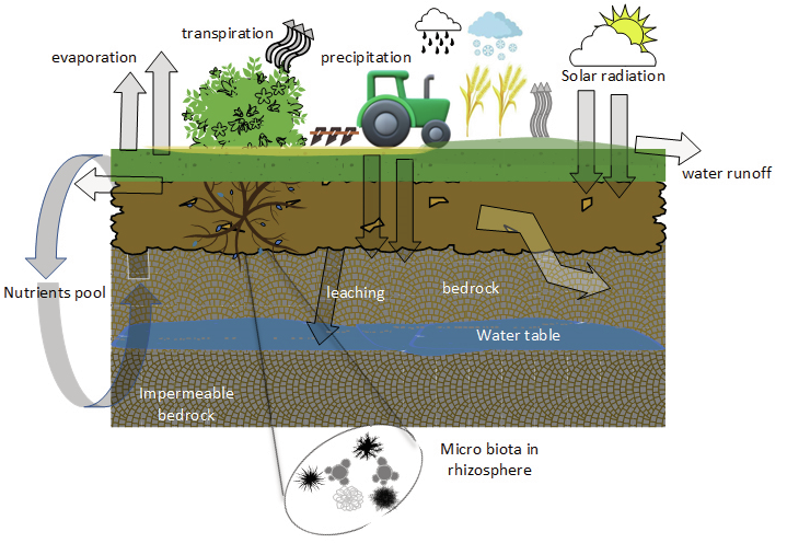
Graphical abstract
Open AccessArticle
Reconstruction of Surface Water Temperature in Lakes as a Source for Long-Term Analysis of Its Changes
by
Mariusz Sojka and Mariusz Ptak
Water 2024, 16(23), 3347; https://doi.org/10.3390/w16233347 (registering DOI) - 21 Nov 2024
Abstract
One of the key parameters of lakes is water temperature, which influences many physical and biochemical processes. In Poland, in situ temperature measurements are or have been conducted in only about 30 lakes, whereas there are over 3000 lakes with an area larger
[...] Read more.
One of the key parameters of lakes is water temperature, which influences many physical and biochemical processes. In Poland, in situ temperature measurements are or have been conducted in only about 30 lakes, whereas there are over 3000 lakes with an area larger than 10 hectares. In many cases, the length of existing observation series is not always sufficient for long-term analysis. Using artificial neural networks of the multilayer perceptron network (MLP) type, the reconstruction of average monthly water temperatures was carried out for nine lakes located in northern Poland. During the validation stage of the reconstruction results, BIAS values were obtained in the range of −0.33 to 0.44 °C, the mean absolute error was 0.46 °C, and the root mean square error was 0.61 °C. The high quality of the reconstructed data allowed for an assessment of water temperature changes in the analyzed lakes from 1993 to 2022 using the Mann–Kendall and Sen tests. It was found that, on an annual basis, the water temperature increased by an average of 0.50 °C per decade, ranging from 0.36 °C per decade to 0.64 °C per decade for individual lakes. For specific months, the largest increase was observed in November, about 0.99 °C per decade, and the smallest in May, 0.07 °C per decade. The obtained results confirm previous studies in this field while adding new data from lakes, which are particularly significant for the western part of Poland—a region with a previously limited number of monitored lakes. According to the findings, the analyzed lakes have undergone significant warming over the past three decades, which is important information for water management authorities.
Full article
(This article belongs to the Special Issue Applications of Artificial Intelligence (AI) in Water Resources Systems)
►▼
Show Figures
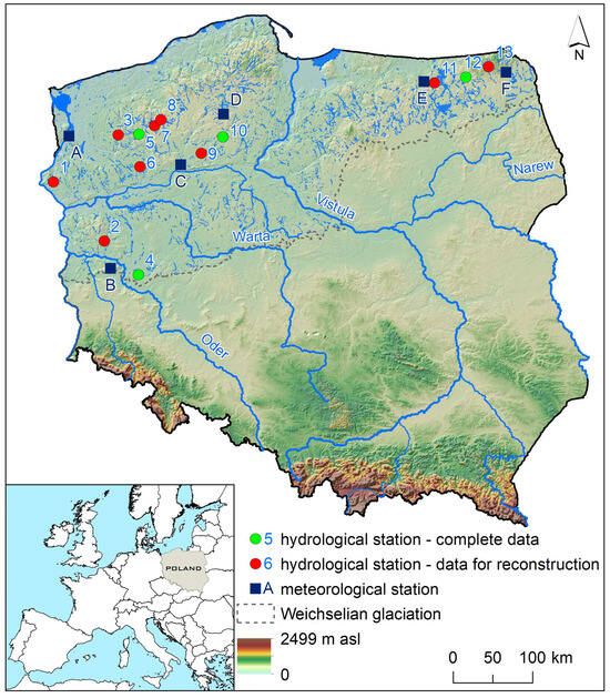
Figure 1
Figure 1
<p>Location of study sites.</p> Full article ">Figure 2
<p>Validation results of MLP-type neural networks presented in a Taylor diagram.</p> Full article ">Figure 3
<p>Variability of mean annual water temperatures in lakes in the period 1993–2022.</p> Full article ">Figure 4
<p>Variability of average monthly water temperatures in Lakes Morzycko and Rospouda Filipowska.</p> Full article ">Figure 5
<p>Changes in average monthly water temperatures in lakes: (<b>a</b>) significance of changes; and (<b>b</b>) value of changes.</p> Full article ">Figure 6
<p>Average change of water temperature regime in Lakes Komorze, Morzycko, Sławianowskie, and Ostrowite.</p> Full article ">
Open AccessArticle
Unveiling the Spatial Variability of Soil Nutrients in Typical Karst Rocky Desertification Areas
by
Dongdong Zhang, Yaying Feng, Bin Zhang, Xinling Fan, Zhen Han and Jinxin Zhang
Water 2024, 16(23), 3346; https://doi.org/10.3390/w16233346 - 21 Nov 2024
Abstract
Soil nutrients are essential for plant survival, especially in karst regions where soil erosion is a significant threat, leading to ecosystem degradation. Rocks exposed in these areas contribute to fragmented soil coverage and the complex spatial distribution of soil nutrients, hindering vegetation recovery.
[...] Read more.
Soil nutrients are essential for plant survival, especially in karst regions where soil erosion is a significant threat, leading to ecosystem degradation. Rocks exposed in these areas contribute to fragmented soil coverage and the complex spatial distribution of soil nutrients, hindering vegetation recovery. In this study, we collected 60 soil samples (0–30 cm deep) from a typical rocky desertification slope. Classical statistics and geostatistics were used to assess the spatial variability of the following key soil properties: soil organic carbon (SOC), total nitrogen (TN), total phosphorus (TP), and total potassium (TK). The study mapped a continuous surface of soil nutrients using the ordinary kriging method to analyze the spatial variability of the karst slope. The results showed that, except for the bulk density and porosity, which showed little variation, the other soil characteristics had moderate to high levels of variability. The SOC, TN, and TP levels decreased with soil depth, while the TK content increased with soil depth. Each soil layer has strong spatial autocorrelation in its SOC. The variability of TP and TK decreases with soil depth, indicating strong spatial autocorrelation. In the 0–10 cm soil layer, the SOC displays the highest level of continuity, with the TN exhibiting a higher level of variability compared to the other nutrients. Within the 10–20 cm soil layer, the SOC, TN, TP, and TK all exhibit strong spatial autocorrelation. Moving to the 20–30 cm soil layer, the structural variability of SOC is the most pronounced. The correlation between soil nutrients and other soil properties was not strong, with only a cumulative explanatory power of 11.81% in the first two axes of a redundancy analysis (RDA). Among them, the bulk density and silt content had a significant impact on soil nutrients. Studying the spatial variability of soil nutrients in rocky desertification areas is crucial for improving soil quality and promoting vegetation restoration.
Full article
(This article belongs to the Special Issue Soil Erosion and Soil and Water Conservation)
►▼
Show Figures
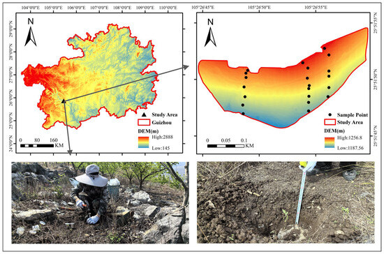
Figure 1
Figure 1
<p>Study area and soil sampling.</p> Full article ">Figure 2
<p>Correlations between physicochemical properties of soil in each layer (where D stands for bulk density, SHC for saturated hydraulic conductivity, SOC for soil organic carbon, TN for total nitrogen, TP for total phosphorus, TK for total potassium, CLAY for clay content, SILT for silt content, and SAND for sand content).</p> Full article ">Figure 3
<p>Spatial distribution of soil nutrients in different soil layers (where SOC represents soil organic carbon, TN represents total nitrogen, TP represents total phosphorus, TK represents total potassium, (<b>a-1</b>–<b>a-4</b>) indicates the 0–10 cm soil layer, (<b>b-1</b>–<b>b-4</b>) indicates the 10–20 cm soil layer, and (<b>c-1</b>–<b>c-4</b>) indicates the 20–30 cm soil layer).</p> Full article ">Figure 4
<p>RDA ranking results.</p> Full article ">
Open AccessArticle
Investigation of Stress Tensor Anisotropy in Two- and Three-Dimensional Dunes
by
Elham Fazel Najafabadi, Hossein Afzalimehr, Mohammad Nazari-Sharabian and Moses Karakouzian
Water 2024, 16(23), 3345; https://doi.org/10.3390/w16233345 - 21 Nov 2024
Abstract
Investigating the creation of bed forms due to sediment transport and flow structure in the presence of bed forms in alluvial channels is a constant challenge for engineers and researchers, because of its complex nature. In this research, turbulent flow structure and turbulence
[...] Read more.
Investigating the creation of bed forms due to sediment transport and flow structure in the presence of bed forms in alluvial channels is a constant challenge for engineers and researchers, because of its complex nature. In this research, turbulent flow structure and turbulence anisotropy in the presence of two- and three-dimensional laboratory dunes were investigated. The results showed that, at the reattachment point, the turbulence anisotropy at the centerline of a three-dimensional dune was the largest. On the stoss slope, the turbulence anisotropy for two-dimensional dunes was at its highest at the bed form’s trough and below the crest. The results also demonstrated a tendency at the crest line toward the plane–strain limit for two-dimensional dunes and the centerline of three-dimensional dunes. However, at a 20 cm distance, turbulence anisotropy at the crest line tended toward asymmetric contraction to an oblate spheroid.
Full article
(This article belongs to the Special Issue Recent Advances in Hydraulics Engineering)
►▼
Show Figures
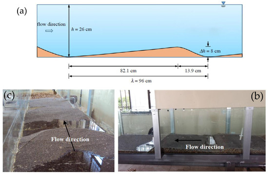
Figure 1
Figure 1
<p>(<b>a</b>) Two-dimensional dune schematic; (<b>b</b>) two- and (<b>c</b>) three-dimensional dunes made in the lab.</p> Full article ">Figure 2
<p>Streamwise velocity profiles in flow over (<b>a</b>) two- and (<b>b</b>) three-dimensional dunes on a vertical central plane, (<b>c</b>) instantaneous velocity for one point in the flow field.</p> Full article ">Figure 3
<p>Reynolds shear stress profiles in flow over (<b>a</b>) two- and (<b>b</b>) three-dimensional dunes on a vertical central plane.</p> Full article ">Figure 4
<p>Anisotropic invariant map (AIM) on −II/III frame (Lumley triangle).</p> Full article ">Figure 5
<p>AIMs at (<b>a</b>) <span class="html-italic">x/λ</span> = 0 (crest); (<b>b</b>) 0.083 (lee slope); (<b>c</b>) 0.146 (trough); (<b>d</b>) 0.224 (on the stoss slope before reattachment point); (<b>e</b>) 0.302 (reattachment point); (<b>f</b>) 0.406 (almost in the middle of the stoss slope); and (<b>g</b>) 0.719 (near the end of the stoss slope) for a two-dimensional dune.</p> Full article ">Figure 6
<p>AIMs at seven non-dimensional streamwise distances, (<b>a</b>) <span class="html-italic">x/λ</span> = 0.104 (stoss slope before crest); (<b>b</b>) 0.417 (crest); (<b>c</b>) 0.521 (lee slope); (<b>d</b>) 0.562 (trough); (<b>e</b>) 0.615 (on the stoss slope before reattachment point); (<b>f</b>) 0.719 (reattachment point); and (<b>g</b>) 0.844 (stoss slope, after reattachment point) for three-dimensional dune centerline.</p> Full article ">Figure 7
<p>AIMs at (<b>a</b>) <span class="html-italic">x/λ</span> = 0.208 (stoss slope before crest); (<b>b</b>) 0.312 (crest); (<b>c</b>) 0.443 (lee slope); (<b>d</b>) 0.457 (trough); (<b>e</b>) 0.469 (on the stoss slope before reattachment point); (<b>f</b>) 0.521 (reattachment point); and (<b>g</b>) 0.719 (stoss slope, after reattachment point) for three-dimensional dune at 20 cm distance from bank channel.</p> Full article ">Figure 8
<p>Anisotropic invariant function <b>F</b> versus nondimensional vertical distance <span class="html-italic">z/h</span> at (<b>a</b>) at the top of the crest, (<b>b</b>) at the lee slope, (<b>c</b>) at the trough, (<b>d</b>) on the stoss slope before the reattachment point, (<b>e</b>) at the reattachment point, (<b>f</b>) on the stoss slope after the reattachment point, (<b>g</b>) on the stoss slope near the slope end. The numbers of 1–3 show a two-dimensional dune, three-dimensional dune centerline, and three-dimensional dune 20 cm distance from the channel bank.</p> Full article ">Figure 9
<p>Data plots for <span class="html-italic">λ<sub>1</sub></span> versus <span class="html-italic">λ<sub>2</sub></span> at (<b>a</b>) the top of the crest, (<b>b</b>) the lee slope, (<b>c</b>) the trough, (<b>d</b>) on the stoss slope before the reattachment point, (<b>e</b>) at the reattachment point, (<b>f</b>) on the stoss slope after the reattachment point, (<b>g</b>) on the stoss slope near the slope end. The numbers 1–3 show two-dimensional dune, three-dimensional dune centerline, and three-dimensional dune 20 cm distance from channel bank.</p> Full article ">
Open AccessArticle
Acidogenic Fermentation of Cassava Wastewater: Effect of the Substrate-to-Microorganism Ratio and Temperature on Volatile Fatty Acids Production
by
Lina Marcela Sanchez-Ledesma, Jenny Alexandra Rodríguez-Victoria and Howard Ramírez-Malule
Water 2024, 16(23), 3344; https://doi.org/10.3390/w16233344 - 21 Nov 2024
Abstract
The production of volatile fatty acids (VFAs) through the acidogenic fermentation of wastewater is an emerging technology that requires further research to optimize operational variables for specific substrates. Cassava wastewater, which is a byproduct of the cassava sour starch extraction process, has been
[...] Read more.
The production of volatile fatty acids (VFAs) through the acidogenic fermentation of wastewater is an emerging technology that requires further research to optimize operational variables for specific substrates. Cassava wastewater, which is a byproduct of the cassava sour starch extraction process, has been minimally studied regarding its potential for VFA production through acidogenic fermentation. Batch reactors were used to evaluate the effects of the substrate-to-microorganism (S/M) ratio and temperature on VFA production from cassava wastewater. The results showed no statistically significant differences between the evaluated S/M ratios. The maximum total VFA concentration observed was 2214.64 mg of acetic acid (HAc)/L (0.32 gCODVFA/gCOD), which was achieved at a S/M ratio of 4 gCOD/gVS. This concentration was predominantly composed of acetic acid (42.7%), followed by butyric acid (30.1%) and propionic acid (24.6%), with a minor quantity of isovaleric acid (2.6%). The statistical analysis for the temperature variable showed significant differences between the evaluated conditions. The maximum concentration of total VFAs was 2650.19 mgHAc/L (0.45 gCODVFA/gCOD) at 34 ± 1 °C, with acetic (40.9%), butyric (29.8%), and propionic (29.3%) acids as primary metabolites. Cassava wastewater shows promise as a potential substrate for VFA production, warranting evaluation in continuous reactors.
Full article
(This article belongs to the Special Issue Water Reuse and Recycling)
►▼
Show Figures
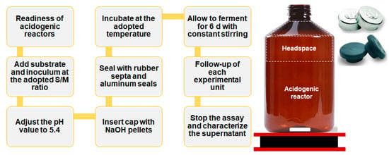
Figure 1
Figure 1
<p>Scheme of the unit and experimental procedure adopted in the AF of CWW.</p> Full article ">Figure 2
<p>Production and yield of VFAs by AF of CWW. (<b>a</b>) Effect of the S/M ratio and (<b>b</b>) effect of the temperature.</p> Full article ">Figure 3
<p>Final carbohydrate concentration and uptake in AF of CWW. (<b>a</b>) Effect of the S/M ratio and (<b>b</b>) effect of the temperature.</p> Full article ">Figure 4
<p>Distribution of VFAs produced in AF of CWW. (<b>a</b>) Effect of the S/M ratio and (<b>b</b>) effect of the temperature.</p> Full article ">Figure 5
<p>Variation of pH and bicarbonate alkalinity in AF of CWW. (<b>a</b>) Effect of the S/M ratio and (<b>b</b>) effect of the temperature.</p> Full article ">
Open AccessArticle
Influence of Filler Types on the Treatment of Rural Domestic Wastewater in a Biological Trickling Filter: Simultaneous Nitrogen and Phosphorus Removal Performance, Microbial Community, and Metabolic Functions
by
Yuxin Geng, Zhengwei Pan, Liangang Hou, Jiarui Li, Mingchao Wang, Tianhao Shi, Dongyue Li and Jun Li
Water 2024, 16(23), 3343; https://doi.org/10.3390/w16233343 - 21 Nov 2024
Abstract
Biological trickling filtration (BTF) has the advantages of simple operation, low energy consumption, and low sludge production, and its application in the treatment of domestic wastewater in rural areas has been widely discussed. In this study, ceramic granule (R1), zeolite (R2), and sponge
[...] Read more.
Biological trickling filtration (BTF) has the advantages of simple operation, low energy consumption, and low sludge production, and its application in the treatment of domestic wastewater in rural areas has been widely discussed. In this study, ceramic granule (R1), zeolite (R2), and sponge (R3), three typical nitrogen and phosphorus removal fillers, were selected to investigate the differences in the removal performance of COD, nitrogen, and phosphorus in BTF, analyze the characteristics of the fillers and biofilm, and determine the performance of simultaneous nitrogen and phosphorus removal. The results show that among the three fillers, zeolite has the larger specific surface area and roughness and has the best treatment effect on the adhesion performance of sewage and biofilm. The richness and diversity of the microbial community are higher, and the system is more stable, with a COD removal rate of 77.10 ± 8.67% and an NH4+-N removal rate of 75.20 ± 6.64%. The TP removal rate was 22.04 ± 10.27%. The surface of ceramic particles showed a regular cluster structure with a loose distribution. The removal rate of COD was 78.49 ± 6.92%, the concentration of NH4+-N in the effluent was 27.95 ± 8.23 mg/L, and the removal rate of TP was 38.83 ± 12.14%. As a polymer composite material, the sponge has large internal pores and a smooth surface, which is not conducive to biofilm adhesion. Therefore, the removal rate of nitrogen and phosphorus in sewage is poor; the removal rate of COD is 75.94 ± 6.98%, NH4+-N is 27.89 ± 21.06%, and the removal rate of TP is 14.07 ± 11.76%. Compared with the metabolic function of genes, zeolites have a more stable enzyme digestion ability than the other two fillers, and the genes related to the nitrification process (amo, hao, nxr, etc.) and functional genes encoding key enzymes related to the TCA cycle are relatively abundant.
Full article
(This article belongs to the Special Issue Sewage Disposal, Biological Processes and Resource Utilization of Sewage Sludge)
►▼
Show Figures
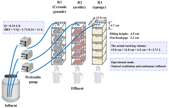
Figure 1
Figure 1
<p>Schematic diagram of biological trickling filter system.</p> Full article ">Figure 2
<p>(<b>a</b>) Physical and SEM images of the three fillers. (<b>b</b>) Biofilm microscopy.</p> Full article ">Figure 3
<p>XRD patterns of fillers. (<b>a</b>) ceramic granule; (<b>b</b>) zeolite; and (<b>c</b>) sponge.</p> Full article ">Figure 4
<p>Performance of simultaneous nitrogen and phosphorus removal; (<b>a</b>,<b>c</b>,<b>e</b>,<b>g</b>) are the inlet and outlet concentrations of COD, NH<sub>4</sub><sup>+</sup>-N, TN, and TP, respectively, and (<b>b</b>,<b>d</b>,<b>f</b>,<b>h</b>) COD, NH<sub>4</sub><sup>+</sup>-N, TN, and TP removal rate, respectively.</p> Full article ">Figure 5
<p>Microbial community structure; (<b>a</b>) phylum level and (<b>b</b>) genus level.</p> Full article ">Figure 6
<p>KEGG pathway analysis in different reactors. (<b>a</b>) Primary classification; (<b>b</b>) secondary classification; (<b>c</b>) third-level classification.</p> Full article ">Figure 7
<p>KEGG prediction of potentially functional genes and enzymes in metabolic pathways of nitrogen metabolism (<b>a</b>), phosphorus metabolism (<b>b</b>), and TCA cycle (<b>c</b>).</p> Full article ">
Open AccessArticle
Trace Elements in Lakes Located in an Agricultural-Forest Catchment: A Case Study of Lake Raczyńskie, Poland
by
Katarzyna Wiatrowska, Jolanta Kanclerz and Ewelina Janicka
Water 2024, 16(23), 3342; https://doi.org/10.3390/w16233342 - 21 Nov 2024
Abstract
The enrichment of bottom sediments with trace elements due to anthropogenic factors is of growing concern worldwide. With the development of industry, agriculture, and urbanization, the risk of freshwater contamination with trace elements is increasing. As trace elements are poorly soluble in water,
[...] Read more.
The enrichment of bottom sediments with trace elements due to anthropogenic factors is of growing concern worldwide. With the development of industry, agriculture, and urbanization, the risk of freshwater contamination with trace elements is increasing. As trace elements are poorly soluble in water, they have a tendency to accumulate in bottom sediments. The study focused on the evaluation of the trace element contents in the surface layer of bottom sediments of Lake Raczyńskie, located in Poland, and assessing the risks posed by these sediments. The pollution of bottom sediments was estimated based on the index of the geo-accumulation (Igeo), enrichment factor (EF), Nemerow multi-factor index (Pn), and pollution load index (PLI). The assessment of environmental risk was evaluated by the potential ecological risk index (RI) and mean PEL quotient method. The results obtained showed that the average contents of Cd, Cu, Ni, Pb, and Zn exceeded the national geochemical background values (Bn), indicating possible enrichment of bottom sediments due to human activity. Only for Mn were the observed contents below the Bn. This evaluation was confirmed by the PLI and Pn values, which indicated sediment pollution from anthropogenic sources. However, the risk assessment by RI and mean PEL showed a low risk of contamination. The results of principal component analysis (PCA) and values of Igeo and EF suggested that Cd, Cu, Mn, and Zn mainly originate from geogenic sources, while Ni and Pb probably come from an unrecognized anthropogenic source. The distribution of Cd, Mn, and Ni depended on the contents of silt and clay fractions. Additionally, organic carbon influenced Cu, Mn, Ni, and Zn contents in bottom sediments.
Full article
(This article belongs to the Section Water Quality and Contamination)
►▼
Show Figures
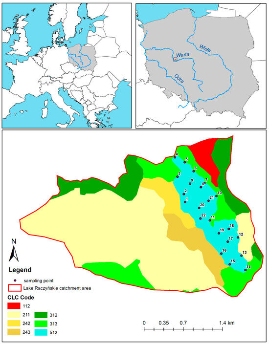
Figure 1
Figure 1
<p>Sampling points in the study area with structure of the land use (112—discontinuous urban fabric; 211—non-irrigated arable land; 242—complex cultivation patterns; 243—land principally occupied by agriculture, with significant areas of natural vegetation; 312—coniferous forest; 313—mixed forest; 512—water bodies) (source: Corine land cover (CLC) vector layers for 2018).</p> Full article ">Figure 2
<p>The local relief of Lake Raczyńskie direct catchment area (digital elevation model (DEM) with bathymetric plan of the lake). A DEM was downloaded with a 1 m by 1 m resolution using LIDAR (light detection and ranging). Sampling points: 1–7, 10–16, 18—bank zone (1–4, 6–7, 10—settlement influence zones; 12–16—agriculture influence zones; 5, 18—tourism influence zones); 8, 9—island zone; 17, 19–22—the central profile of the lake. The bathymetric plan was obtained from the resources of the National Inland Fisheries Research Institute, which was vectorized in the ArcGIS program ver. 10.8.1.</p> Full article ">Figure 3
<p>Spatial distribution of trace elements in the surface sediment of Lake Raczyńskie, Poland. (<b>a</b>) Cd content; (<b>b</b>) Cu content; (<b>c</b>) Mn content; (<b>d</b>) Ni content; (<b>e</b>) Pb content; (<b>f</b>) Zn content.</p> Full article ">Figure 3 Cont.
<p>Spatial distribution of trace elements in the surface sediment of Lake Raczyńskie, Poland. (<b>a</b>) Cd content; (<b>b</b>) Cu content; (<b>c</b>) Mn content; (<b>d</b>) Ni content; (<b>e</b>) Pb content; (<b>f</b>) Zn content.</p> Full article ">Figure 4
<p>The values of I<sub>geo</sub> in the bottom sediments of Lake Raczyńskie.</p> Full article ">Figure 5
<p>The values of mean PEL-Q of the bottom sediments of Lake Raczyńskie.</p> Full article ">Figure 6
<p>Loading plot of trace elements in the space defined by PC1 and PC2.</p> Full article ">
Open AccessArticle
Deformation Modeling and Prediction of Concrete Dam Using Observed Air Temperature and Enhanced CatBoost Algorithm
by
Fang Xing, Hui Li and Tianyu Li
Water 2024, 16(23), 3341; https://doi.org/10.3390/w16233341 - 21 Nov 2024
Abstract
Accurate prediction of concrete dam deformation is essential for ensuring structural safety and operational efficiency. This study presents a novel approach for monitoring and predicting concrete dam deformation using observed air temperature data, intelligent optimization, and machine learning techniques. To address the limitations
[...] Read more.
Accurate prediction of concrete dam deformation is essential for ensuring structural safety and operational efficiency. This study presents a novel approach for monitoring and predicting concrete dam deformation using observed air temperature data, intelligent optimization, and machine learning techniques. To address the limitations of traditional statistical models in simulating the thermal effects on dam body deformation, this study proposes an improved hydraulic–air temperature–time (HTairT) deformation monitoring model. This model leverages long-term air temperature data and its lagged terms as critical input variables, enabling a more comprehensive understanding of thermal impacts on dam deformation. To capture the complex, nonlinear relationships between environmental factors and dam deformation behavior, we introduce the high-performance CatBoost gradient-boosting algorithm as a regressor. An enhanced Particle Swarm Optimization (PSO) algorithm is utilized for optimizing CatBoost’s parameters, enhancing the model’s predictive accuracy. A high concrete dam, currently in service, is selected as the case study, where two representative deformation monitoring points are used for validation. This research fills a gap by combining CatBoost with an optimized PSO in a deformation monitoring model, providing a novel approach that improves predictive reliability in long-term dam safety monitoring. Experimental results show that the enhanced PSO-optimized CatBoost algorithm achieves higher R2 and lower MSE and MAE values in multiple monitoring points. compared with other benchmark methods Moreover, the importance of factors affecting deformation can be identified using the proposed method, and experimental results indicate that water level and average air temperature of 1–2 days, 3–7 days, and 30–60 days are key factors affecting the deformation of high concrete arch dams.
Full article
(This article belongs to the Section Hydraulics and Hydrodynamics)
►▼
Show Figures
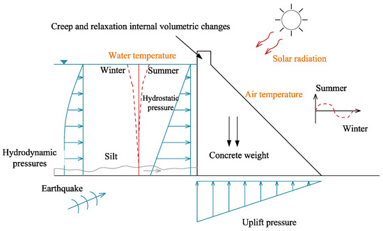
Figure 1
Figure 1
<p>Schematic diagram of the environmental loads during the service period.</p> Full article ">Figure 2
<p>Intuitive diagram of CatBoost regression model.</p> Full article ">Figure 3
<p>Intuitive diagram of position update mechanism in PSO algorithms.</p> Full article ">Figure 4
<p>Calculation process of improved PSO optimization algorithm.</p> Full article ">Figure 5
<p>Dam deformation monitoring system.</p> Full article ">Figure 6
<p>Concrete dam deformation change process line.</p> Full article ">Figure 7
<p>Concrete dam temperature and hysteresis process line.</p> Full article ">Figure 8
<p>Comparison of prediction performance on the test set using different input factors.</p> Full article ">Figure 9
<p>Changes in negative MSE during model parameter optimization.</p> Full article ">Figure 10
<p>Multi-index changes during model parameter optimization.</p> Full article ">Figure 11
<p>Prediction results and residual analysis of different methods.</p> Full article ">Figure 12
<p>Radar chart analysis of prediction results of different regression algorithms Comparison of residual box plots of different prediction methods.</p> Full article ">Figure 13
<p>Importance analysis of factors affecting dam deformation.</p> Full article ">
Open AccessArticle
Effect of Rainfall and Water Level Rise and Fall on Stability of Core Wall Embankment
by
Wei Zhao, Haoyu Mao, Lingfeng Sun, Xujiang Lu and Shulin Sun
Water 2024, 16(23), 3340; https://doi.org/10.3390/w16233340 - 21 Nov 2024
Abstract
►▼
Show Figures
Transient seepage triggered by rainfall and water level changes has a significant impact on embankment stability. To investigate the effects of rainfall and water level changes on the seepage field of embankments, numerical comparative experiments were conducted based on the Shu River embankment
[...] Read more.
Transient seepage triggered by rainfall and water level changes has a significant impact on embankment stability. To investigate the effects of rainfall and water level changes on the seepage field of embankments, numerical comparative experiments were conducted based on the Shu River embankment project. The influence of key factors such as rainfall, water level rise and fall rate, and rainfall-coupled water level rise and fall on the internal seepage field of the embankment was analyzed, and the main factors affecting the stability of the embankment slope were identified. The relationship among permeability coefficient, lag rate of the phreatic line, and embankment slope stability factor is explored, and fitting equations are developed. The results show that rainfall infiltration increases the pore water pressure of the soil, leading to a decrease in the effective stress of the soil and a decrease in the slope stability factor. The stability factor of the embankment slope is positively correlated with the rise and fall of the water level, and the faster the rate of rise and fall, the higher the rate of change in pore water pressure. The stability factor of the embankment slope showed a trend of decreasing and then increasing with the decrease in water level, and when the water level had decreased by 70%, the lag rate of the phreatic line was the largest, and the stability factor of the embankment slope was the lowest. The established equations for fitting the stability factor of the embankment slope to the lag rate of the phreatic line can be used as a reference for the safety assessment of similar embankment projects.
Full article
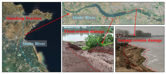
Figure 1
Figure 1
<p>Seepage failure phenomenon of sandy embankments along the Shuhe River.</p> Full article ">Figure 2
<p>Core wall embankment structure and monitoring point layout</p> Full article ">Figure 3
<p>Monthly rainfall distribution in the study area.</p> Full article ">Figure 4
<p>The curve of volumetric water content and matric suction for the core wall embankment.</p> Full article ">Figure 5
<p>Rainfall infiltration seepage vector diagrams at low water level.</p> Full article ">Figure 6
<p>The variation curves of pore water pressure at each monitoring point in Plan <span class="html-italic">A</span><sub>1</sub><b>.</b></p> Full article ">Figure 7
<p>Rainfall infiltration seepage vector diagrams at high water level.</p> Full article ">Figure 8
<p>The variation curves of pore water pressure at each monitoring point in Plan <span class="html-italic">A</span><sub>2</sub>.</p> Full article ">Figure 9
<p>Seepage vector diagrams of water level rise and fall.</p> Full article ">Figure 10
<p>Seepage vector diagram of the core wall embankment when the water level is at 9 m</p> Full article ">Figure 11
<p><span class="html-italic">P</span><sub>3</sub> and <span class="html-italic">H</span><sub>3</sub>-pore water pressure variation curves under different water level rise and fall rates.</p> Full article ">Figure 12
<p>Seepage vector diagrams under rising water level coupled with rainfall. (<b>a</b>) Vectors of seepage flow at different rates of rise. (<b>b</b>) Vectors of seepage under coupled rainfall with different rise rates.</p> Full article ">Figure 13
<p>Variation curves of the pore water pressure at measurement points <span class="html-italic">P<sub>i</sub></span> and <span class="html-italic">H<sub>i</sub></span> under coupled water level fluctuations and rainfall effects.</p> Full article ">Figure 13 Cont.
<p>Variation curves of the pore water pressure at measurement points <span class="html-italic">P<sub>i</sub></span> and <span class="html-italic">H<sub>i</sub></span> under coupled water level fluctuations and rainfall effects.</p> Full article ">Figure 14
<p>Graph of the variation in embankment slope stability factor under rising water levels and the combined effects of rising water levels and rainfall.</p> Full article ">Figure 15
<p>Variation curves of the slope stability factor under water level drawdown and rainfall conditions.</p> Full article ">Figure 16
<p>Variation curves of slope stability factor and changes in permeability coefficient.</p> Full article ">Figure 17
<p>Variation curves of the relationships between slope stability factor and permeability coefficient, and between slope stability factor and phreatic line lag rate.</p> Full article ">
Open AccessArticle
Unveiling the Intra-Annual and Inter-Annual Spatio-Temporal Dynamics of Sediment Inflow to Rivers and Driving Factors in Cloud-Prone Regions: A Case Study in Minjiang River Basin, China
by
Xiaoqin Wang, Zhichao Yu, Lin Li, Mengmeng Li, Jinglan Lin, Lifang Tang, Jianhui Chen, Haihan Lin, Miao Chen, Shilai Jin, Yunzhi Chen and Xiaocheng Zhou
Water 2024, 16(22), 3339; https://doi.org/10.3390/w16223339 - 20 Nov 2024
Abstract
Accurately delineating sediment export dynamics using high-quality vegetation factors remains challenging due to the spatio-temporal resolution imbalance of single remote sensing data and persistent cloud contamination. To address these challenges, this study proposed a new framework for estimating and analyzing monthly sediment inflow
[...] Read more.
Accurately delineating sediment export dynamics using high-quality vegetation factors remains challenging due to the spatio-temporal resolution imbalance of single remote sensing data and persistent cloud contamination. To address these challenges, this study proposed a new framework for estimating and analyzing monthly sediment inflow to rivers in the cloud-prone Minjiang River Basin. We leveraged multi-source remote sensing data and the Continuous Change Detection and Classification model to reconstruct monthly vegetation factors at 30 m resolution. Then, we integrated the Chinese Soil Loss Equation model and the Sediment Delivery Ratio module to estimate monthly sediment inflow to rivers. Lastly, the Optimal Parameters-based Geographical Detector model was harnessed to identify factors affecting sediment export. The results indicated that: (1) The simulated sediment transport modulus showed a strong coefficient of determination (R2 = 0.73) and a satisfactory Nash–Sutcliffe efficiency coefficient (0.53) compared to observed values. (2) The annual sediment inflow to rivers exhibited a spatial distribution characterized by lower levels in the west and higher in the east. The monthly average sediment value from 2016 to 2021 was notably high from March to July, while relatively low from October to January. (3) Erosive rainfall was a decisive factor contributing to increased sediment entering the rivers. Vegetation factors, manifested via the quantity (Fractional Vegetation Cover) and quality (Leaf Area Index and Net Primary Productivity) of vegetation, exert a pivotal influence on diminishing sediment export.
Full article
(This article belongs to the Special Issue The Interrelationship Between Climate Change, Human Activities and Hydrological Processes (3rd Edition))
►▼
Show Figures
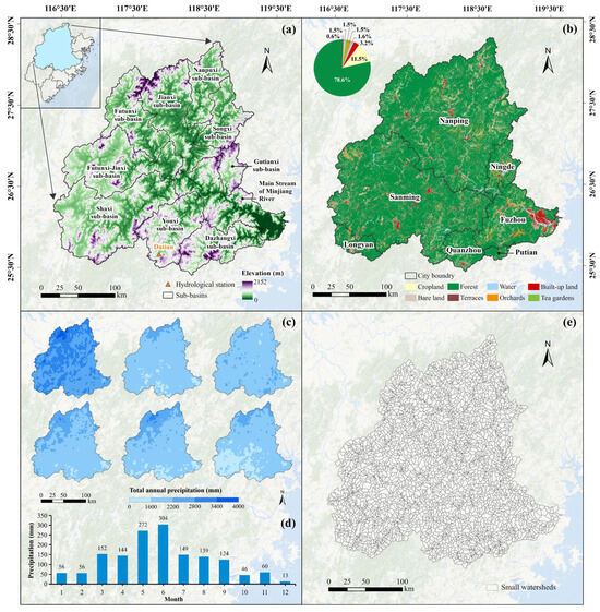
Figure 1
Figure 1
<p>Overview of the study region. (<b>a</b>) Location of the study area in Fujian; (<b>b</b>) Land use in 2021; (<b>c</b>) Total annual precipitation from 2016 to 2021; (<b>d</b>) Multi-year monthly average precipitation from 2016 to 2021; (<b>e</b>) Delineation of small watersheds in the MJRB.</p> Full article ">Figure 2
<p>Available monthly observations of GF-1 WFV, Landsat-8 OLI, Sentinel-2 MSI with cloud cover less than 10% from 2016 to 2021.</p> Full article ">Figure 3
<p>An overview of the workflow in this study (Notes: *: <span class="html-italic">p</span> < 0.05; ***: <span class="html-italic">p</span> < 0.001).</p> Full article ">Figure 4
<p>Spatial distribution of driving factors in 2021. (<b>a</b>) FVC; (<b>b</b>) LAI; (<b>c</b>) NPP; (<b>d</b>) BRI; (<b>e</b>) PF; (<b>f</b>) PT; (<b>g</b>) HAILS; (<b>h</b>) LRR; (<b>i</b>) PB.</p> Full article ">Figure 5
<p>Validation of the model estimation results.</p> Full article ">Figure 6
<p>Demonstrations of turbidity change for typical river sections from 2016 to 2021. (<b>1</b>) River section located in the upper reaches of the MJRB within the Futunxi-Jinxi sub-basin; (<b>2</b>) River section situated in the midstream within the Gutianxi sub-basin; (<b>3</b>) Main stream of the Minjiang River in the lower reaches.</p> Full article ">Figure 7
<p>Proportion of different turbidity for river sections from 2016 to 2021.</p> Full article ">Figure 8
<p>Distribution of sediment inflow to rivers from 2016 to 2021.</p> Full article ">Figure 9
<p>Statistics of annual sediment inflow to rivers for small watersheds from 2016 to 2021. The bottom and top edges of the boxes indicate the 25th and 75th percentiles, respectively. The horizontal bold blue lines denote the median. The dashed lines extended from the interquartile with length of 1.5 times box width. The dots represent the mean.</p> Full article ">Figure 10
<p>Spatial distribution of annual sediment inflow to rivers from 2016 to 2021. (Noted: The values presented represent the actual annual sediment load).</p> Full article ">Figure 11
<p>Spatial distribution of annual average sediment inflow to rivers (<b>a</b>) and annual average sediment influx ratio to rivers (<b>b</b>) from 2016 to 2021.</p> Full article ">Figure 12
<p>Overview of the Gutianxi sub-basin. (<b>a</b>) Elevation of the Gutianxi sub-basin; (<b>b</b>) High-resolution remote sensing image from Google Earth.</p> Full article ">Figure 13
<p>Distribution of monthly average sediment inflow to rivers from 2016 to 2021.</p> Full article ">Figure 14
<p>Statistics of monthly average sediment inflow to rivers for small watersheds from 2016 to 2021. The bottom and top edges of the boxes indicate the 25th and 75th percentiles, respectively. The horizontal bold blue lines denote the median. The dashed lines extended from the interquartile with length of 1.5 times box width. The dots represent the mean.</p> Full article ">Figure 15
<p>Multi-year monthly average sediment inflow to rivers and erosive rainfall/R factor from 2016 to 2021.</p> Full article ">Figure 16
<p>Correlation between sediment inflow to rivers and other factors from 2016 to 2021 (Notes: SR: Sediment inflow to Rivers; FVC: Fractional Vegetation Coverage; LAI: Leaf Area Index; NPP: Net Primary Productivity; BRI: Biological Richness Index; PF: Proportion of Forest Land; ER: erosive rainfall; HAILS: Human Activity Intensity of Land Surface; LRR: Land Reclamation Rate; PB: Proportion of Built-up land; *: <span class="html-italic">p</span> < 0.05; ***: <span class="html-italic">p</span> < 0.001).</p> Full article ">Figure 17
<p>Spatial distribution of dominant factor to sediment inflow to rivers (<b>a</b>) and contribution (q-value) of different factors to sediment inflow to rivers (<b>b</b>) from 2016 to 2021.</p> Full article ">Figure 18
<p>Spatial distribution of dominant factor combinations to sediment inflow to rivers.</p> Full article ">Figure 19
<p>Multi-year monthly average FVC and B factor from 2016 to 2021.</p> Full article ">Figure 20
<p>Comparison of measured sediment transport modulus with simulated values calculated separately using the CSLE + SDR and RUSLE + SDR models.</p> Full article ">
Open AccessArticle
A Stable Isotope Analysis to Quantify the Contribution of Basal Dietary Sources to Food Webs of Drinking Water Reservoirs
by
Feng Huang, Wen Zhao, Xingye Qiao, Changge Xia, Yuan Liu, Jie Wei, Dongpeng Yin and George Arhonditsis
Water 2024, 16(22), 3338; https://doi.org/10.3390/w16223338 - 20 Nov 2024
Abstract
►▼
Show Figures
This study investigates the food web structure of the Xinlicheng Reservoir, a drinking water source of critical importance in Changchun, China, by employing stable isotope analysis (SIA) to quantify the contribution ratios of four basal dietary sources—phytoplankton, zooplankton, sediment organic matter, and particulate
[...] Read more.
This study investigates the food web structure of the Xinlicheng Reservoir, a drinking water source of critical importance in Changchun, China, by employing stable isotope analysis (SIA) to quantify the contribution ratios of four basal dietary sources—phytoplankton, zooplankton, sediment organic matter, and particulate organic matter (POM)—to the diets of two key filter-feeding fish species, Hypophthalm ichthys molitrix and Aristichthys nobilis. The analysis reveals that phytoplankton is the dominant dietary source for both species, contributing 32.08% and 34.06%, respectively, whereas the POM contribution is discernably lower (13.25%). The average trophic level of the fish assemblage in Xinlicheng Reservoir is 3.03, while the trophic levels of the two filter-feeding species lie between 3.00 and 3.50. Furthermore, a random forest model was used to identify key environmental drivers of isotopic variations in these basal dietary sources, highlighting the significant role of pH, total nitrogen (TN), chloride (Cl−), calcium (Ca2+), phosphorus (TP), and silicate (
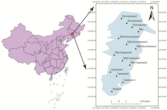
Figure 1
Figure 1
<p>Geographic locations of study sites and sampling stations.</p> Full article ">Figure 2
<p>Spatial distribution of carbon and nitrogen stable isotope values of the four major basal dietary sources in the Xinlicheng Reservoir. Locations within the reservoir, upstream, midstream-upper, midstream-lower, downstream, wetland, and bay are sequentially labeled with numbers 1–6. The lines divide the niche map into four quadrants (<b>A</b>–<b>D</b>).</p> Full article ">Figure 3
<p>Trophic levels of fish in the Xinlicheng Reservoir.</p> Full article ">Figure 4
<p>Box plots of the percentage contribution of four major basal dietary sources to the diet of <span class="html-italic">H. molitrix</span>.</p> Full article ">Figure 5
<p>Box plots of the percentage contribution of four major basal dietary sources to the diet of <span class="html-italic">A. nobilis</span>.</p> Full article ">Figure 6
<p>Box plots showing the percentage contribution of the four major basal dietary sources to the diet of <span class="html-italic">H. molitrix</span> across different locations within Xinlicheng Reservoir.</p> Full article ">Figure 7
<p>Box plots showing the percentage contribution of the four major basal dietary sources to the diet of <span class="html-italic">A. nobilis</span> across different locations within Xinlicheng Reservoir.</p> Full article ">Figure 8
<p>Order of importance of environmental factors related to carbon (<b>A</b>) and nitrogen (<b>B</b>) isotopic signatures of phytoplankton and partial dependence plots of key environmental factors (<b>C</b>: pH; <b>D</b>: TN).</p> Full article ">Figure 9
<p>Order of importance of environmental factors related to carbon (<b>A</b>) and nitrogen (<b>B</b>) isotopes of zooplankton and partial dependence plots of key environmental factors (<b>C</b>: Cl<sup>−</sup>; <b>D</b>: Ca<sup>2+</sup>).</p> Full article ">Figure 10
<p>Order of importance of environmental factors related to carbon (<b>A</b>) and nitrogen (<b>B</b>) isotopes of particulate organic matter and partial dependence plots of key environmental factors (<b>C</b>: SiO<sub>4</sub><sup>4−</sup>; <b>D</b>: pH).</p> Full article ">Figure 11
<p>Order of importance of environmental factors related to carbon (<b>A</b>) and nitrogen (<b>B</b>) isotopes of bottom sediment organic matter and partial dependence plots of key environmental factors (<b>C</b>: TP; <b>D</b>: SO<sub>4</sub><sup>2−</sup>).</p> Full article ">
Open AccessArticle
Effects of Forest Operations on Runoff and Sediment Variations in Catchments Under Intense Forest Activity and Climate Stress in the South-Central Chile
by
Daniel Sanhueza, Giacomo Pellegrini, Andrés Iroumé and Lorenzo Picco
Water 2024, 16(22), 3337; https://doi.org/10.3390/w16223337 - 20 Nov 2024
Abstract
Forestry operations and climate variability affect hydrologic response and sediment transport. Management of forested catchments under intense forestry activity in areas under climatic stress is critical. This study analyzes the impact of forest operations (thinning and clearcutting) on runoff (Q) and suspended sediment
[...] Read more.
Forestry operations and climate variability affect hydrologic response and sediment transport. Management of forested catchments under intense forestry activity in areas under climatic stress is critical. This study analyzes the impact of forest operations (thinning and clearcutting) on runoff (Q) and suspended sediment loads (SSL) in three small catchments (named N02, N03 and N04, respectively) in south-central Chile, where rainfall has decreased by 20% since 2010. Using modified double mass curves and piecewise regression, we separated the effects of forest practices and climate. Thinning in N02 initially reduced Q and SSL, with stable Q overtime, while final harvest in N03 and N04 increased Q, although less than expected. SSL surged post-harvest: 3.6 times in N03 and 1.8 times in N04, potentially linked to hillslope instability. Major SSL events contributed over 55% of post-harvest sediment yield in both catchments, with maximum yields reaching 7.2 tons ha−1 yr−1 in N03 and 4.1 tons ha−1 yr−1 in N04. SSL recovered to pre-harvest levels by the third year, except during a rainy year. Management practices likely contributed to lower SSL and faster recovery. These findings improve our understanding of catchment responses to forest practices and climate change, aiding sustainable forest and water resource management.
Full article
(This article belongs to the Special Issue Catchment Hydrology under Climate Change)
►▼
Show Figures
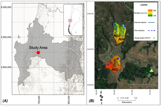
Figure 1
Figure 1
<p>(<b>A</b>) Study area location; the gray area represents the administrative boundary of the Biobío Region in Chile. (<b>B</b>) Forested catchments selected for the study.</p> Full article ">Figure 2
<p>Annual PP and PET in the study area; gray bars represent total PP, violet segmented line represents the historical average, blue segmented line represents the mean PP for the 2010–2019 period (1186 mm yr<sup>−1</sup>) and red segmented lines represent mean PET for the 2008–2010 period (1239 mm yr<sup>−1</sup>) and the 2010–2019 period (1322 mm yr<sup>−1</sup>). Pre-drought (2008–2010) and drought (2010–2019) conditions were represented with different colors and delimited with a black segmented line.</p> Full article ">Figure 3
<p>(<b>A</b>) Monthly PP and PET totals in the study area. The black and red segmented lines represent the linear trends of PP and PET over time, respectively. (<b>B</b>) Monthly PP and PET means in the study area. Pre- and post-(drought) monthly means are represented by continuous and segmented lines, respectively. The dotted lines delimit the periods corresponding to the dry (grey boxes) and wet (blue box) seasons according to the hydrological year in the study area.</p> Full article ">Figure 4
<p>Monthly cumulative difference between PP and PET from pre drought to drought conditions and in the study area. Black dots represent the value of the cumulative difference between PP and PET, and the red line represents the fluctuation between the values.</p> Full article ">Figure 5
<p>(<b>A</b>,<b>C</b>,<b>E</b>) are modified double mass curves (MDMCs) with the accumulated monthly runoff (Qa) plotted against the accumulated monthly effective precipitation (ePa) for N02, N03 and N04, respectively; red lines represent the data recorded before the break points (BP) in the curves, continuous black lines represent the data recorded after the BP, black segmented lines represent predicted values and the linear equation of the data before BP is presented. (<b>B</b>,<b>D</b>,<b>F</b>) are monthly runoff (Q) records for N02, N03 and N04 respectively; black lines represent monthly runoff, red segmented lines represent month of operations and yellow segmented lines represent the month of the BP from MDMC’s analysis.</p> Full article ">Figure 6
<p>Accumulated monthly runoff deviation (ΔQa) and its components for each catchment N02 (<b>A</b>), N03 (<b>B</b>) and N04 (<b>C</b>). ΔQa, accumulated monthly streamflow deviation; ΔQaf, accumulated forest operations effect; ΔQac, accumulated climatic effect.</p> Full article ">Figure 7
<p>(<b>A</b>,<b>C</b>,<b>E</b>) are MDMCs with the accumulated monthly suspended sediment load (mSSLa) plotted against the accumulated monthly runoff (Qa) for N02, N03 and N04, respectively; red lines represent the data recorded before the BP, continuous black lines represent the data recorded after the BP, black segmented lines represent predicted values and the linear equation of the data before BP is presented. (<b>B</b>,<b>D</b>,<b>F</b>) are monthly suspended sediment load (mSSL) records for N02, N03 and N04, respectively; black lines represent mSSL, red segmented lines represent month of operations and yellow segmented lines represent the month of the BP from the MDMCs analysis.</p> Full article ">Figure 8
<p>(<b>A</b>–<b>C</b>) are the total accumulated monthly SSL deviation (ΔmSSLa) and its components, total monthly deviation associated to forest operations (ΔmSSLaf) and total monthly deviation associated to climate variability (ΔmSSLac) for N02, N03 and N04, respectively.</p> Full article ">
Open AccessArticle
Optimization of Ecological Dispatch and Hydrodynamic Improvements in Tidal River Channels Using SWMM Modeling: A Case Study of the Longjin Yangqi Area in Kurama Mountain
by
Wentao Zhou and Weihong Liao
Water 2024, 16(22), 3336; https://doi.org/10.3390/w16223336 - 20 Nov 2024
Abstract
Being tidal-sensitive, the river channel in the Longjin Yangqi area of Cangshan, Fuzhou City, is challenged further because of rapid urbanization. Thus, resultant remediation efforts are crucial. This study aims analyzes hydrodynamic characteristics of the area and, secondly, proposes an ecological dispatch solution
[...] Read more.
Being tidal-sensitive, the river channel in the Longjin Yangqi area of Cangshan, Fuzhou City, is challenged further because of rapid urbanization. Thus, resultant remediation efforts are crucial. This study aims analyzes hydrodynamic characteristics of the area and, secondly, proposes an ecological dispatch solution with evaluation of its effectiveness through the Storm Water Management Model (SWMM). The chief tasks cover imitating rainfall runoff, optimizing sluice gate activities, reorganizing pump management, and reshaping river morphology to bolster flood control and water quality. Improvements were shown through ecological dispatch strategies, which suggested increasing the channel width for the river and deepening the riverbed, thereby increasing the flood duration, lowering water levels, and less frequent flood occurrences. Optimizing sluice gate settings improved efficiency in the regulation of water flow and reduced scour or siltation problems. Various adjustments to pumping operations scattered over various times were based on live-data analysis, therefore enhancing water flow and the self-purification capacity of the water body. The SWMM was directly applied in this tidal river for urban water resource management with data processing from over 100,000 points in simulations. Wherever needed, changes to model parameters were made to improve its capability and enhance its appropriate use in future urban settings. As a whole, this study presents a plan for sustainable water resource management paired with environmental conditions for the benefit of over 500,000 urban residents in the Longjin Yangqi area.
Full article
(This article belongs to the Section Hydraulics and Hydrodynamics)
►▼
Show Figures
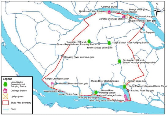
Figure 1
Figure 1
<p>Overview of the study area.</p> Full article ">Figure 2
<p>Flow chart of water quality optimization function.</p> Full article ">Figure 3
<p>High and low tidal variability in 2021.</p> Full article ">Figure 4
<p>Schematic diagram of the scheduling process in the Yangqi area.</p> Full article ">Figure 5
<p>Flow velocity of the Mazhou and Wushan Rivers during periods of high water abundance.</p> Full article ">Figure 6
<p>Flow velocity of Mazhou River and Wushan River during dry water period.</p> Full article ">Figure 7
<p>Flow velocity of Baihu Ting River and Longjin Leapfrog Connected River during abundant water period.</p> Full article ">Figure 8
<p>Flow velocity of Baihu Ting River and Longjin Leapfrog Connecting River during dry water period.</p> Full article ">Figure 9
<p>Changes in ammonia nitrogen concentrations in the Mazhou River after optimization of the abundance period.</p> Full article ">Figure 10
<p>Changes in ammonia nitrogen concentration after optimization of abundant water in Wushan River.</p> Full article ">Figure 11
<p>Changes in ammonia nitrogen concentration in the Mazhou River after dry period optimization.</p> Full article ">Figure 12
<p>Changes in ammonia nitrogen concentrations before and after dry period optimization in the Wushan River.</p> Full article ">Figure 13
<p>Changes in ammonia nitrogen Concentrations after remediation of the Ma Chau River monitoring section.</p> Full article ">Figure 14
<p>Changes in concentration of ammonia nitrogen at the monitoring section of Wushan River.</p> Full article ">
Open AccessArticle
Improving Hydrological Simulations with a Dynamic Vegetation Parameter Framework
by
Haiting Gu, Yutai Ke, Zhixu Bai, Di Ma, Qianwen Wu, Jiongwei Sun and Wanghua Yang
Water 2024, 16(22), 3335; https://doi.org/10.3390/w16223335 - 20 Nov 2024
Abstract
Many hydrological models incorporate vegetation-related parameters to describe hydrological processes more precisely. These parameters should adjust dynamically in response to seasonal changes in vegetation. However, due to limited information or methodological constraints, vegetation-related parameters in hydrological models are often treated as fixed values,
[...] Read more.
Many hydrological models incorporate vegetation-related parameters to describe hydrological processes more precisely. These parameters should adjust dynamically in response to seasonal changes in vegetation. However, due to limited information or methodological constraints, vegetation-related parameters in hydrological models are often treated as fixed values, which restricts model performance and hinders the accurate representation of hydrological responses to vegetation changes. To address this issue, a vegetation-related dynamic-parameter framework is applied on the Xinanjiang (XAJ) model, which is noted as Eco-XAJ. The dynamic-parameter framework establishes the regression between the Normalized Difference Vegetation Index (NDVI) and the evapotranspiration parameter K. Two routing methods are used in the models, i.e., the unit hydrograph (XAJ-UH and Eco-XAJ-UH) and the Linear Reservoir (XAJ-LR and Eco-XAJ-LR). The original XAJ model and the modified Eco-XAJ model are applied to the Ou River Basin, with detailed comparisons and analyses conducted under various scenarios. The results indicate that the Eco-XAJ model outperforms the original model in long-term discharge simulations, with the NSE increasing from 0.635 of XAJ-UH to 0.647 of Eco-XAJ-UH. The Eco-XAJ model also reduces overestimation and incorrect peak flow simulations during dry seasons, especially in the year 1991. In drought events, the modified model significantly enhances water balance performance. The Eco-XAJ-UH outperforms the XAJ-UH in 9 out of 16 drought events, while the Eco-XAJ-LR outperforms the XAJ-LR in 14 out of 16 drought events. The results demonstrate that the dynamic-parameter model, in regard to vegetation changes, offers more accurate simulations of hydrological processes across different scenarios, and its parameters have reasonable physical interpretations.
Full article
(This article belongs to the Special Issue Advances in Machine Learning and Artificial Intelligence Technologies for Hydrological Processes and Hydrologic Disasters)
►▼
Show Figures
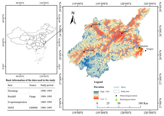
Figure 1
Figure 1
<p>Location and basic information for the Ou River basin.</p> Full article ">Figure 2
<p>Flowchart of the study.</p> Full article ">Figure 3
<p>Procedure of building the Eco-XAJ model.</p> Full article ">Figure 4
<p>Scatter plot of K and the NDVI: (<b>a</b>,<b>b</b>) represent the XAJ-UH model and (<b>c</b>,<b>d</b>) represent the XAJ-LR model. <math display="inline"><semantics> <mrow> <msub> <mrow> <mi mathvariant="normal">N</mi> <mi mathvariant="normal">D</mi> <mi mathvariant="normal">V</mi> <mi mathvariant="normal">I</mi> </mrow> <mrow> <mi mathvariant="normal">t</mi> </mrow> </msub> </mrow> </semantics></math> and <math display="inline"><semantics> <mrow> <msub> <mrow> <mi mathvariant="normal">K</mi> </mrow> <mrow> <mi mathvariant="normal">t</mi> </mrow> </msub> </mrow> </semantics></math> indicate the relationship for the same month; <math display="inline"><semantics> <mrow> <msub> <mrow> <mi mathvariant="normal">N</mi> <mi mathvariant="normal">D</mi> <mi mathvariant="normal">V</mi> <mi mathvariant="normal">I</mi> </mrow> <mrow> <mi mathvariant="normal">t</mi> <mo>−</mo> <mn>1</mn> </mrow> </msub> </mrow> </semantics></math> and <math display="inline"><semantics> <mrow> <msub> <mrow> <mi mathvariant="normal">K</mi> </mrow> <mrow> <mi mathvariant="normal">t</mi> </mrow> </msub> </mrow> </semantics></math> indicate the relationship with a one-month lag.</p> Full article ">Figure 5
<p>Hydrograph of the Eco-XAJ-UH model in (<b>a</b>) the full period, (<b>b</b>) Duration I (the wet season), (<b>c</b>) Duration II (the dry season), and (<b>d</b>) Duration III (the recession periods).</p> Full article ">Figure 6
<p>Hydrograph of the Eco-XAJ-LR model in (<b>a</b>) the full period, (<b>b</b>) Duration I (the wet season), (<b>c</b>) Duration II (the dry season), and (<b>d</b>) Duration III (the recession periods).</p> Full article ">Figure 7
<p>Comparison of the simulation (<b>a</b>,<b>b</b>) between the XAJ-UH model and the Eco-XAJ-UH model, and (<b>c</b>,<b>d</b>) between the XAJ-LR model and the Eco-XAJ-LR model.</p> Full article ">Figure 8
<p>(<b>a</b>,<b>c</b>) are scatter plots of corresponding discharge errors, while (<b>b</b>,<b>d</b>) show scatter plots and the cumulative ∆Error when the observed discharge is below 1000 m<sup>3</sup>/s, where <math display="inline"><semantics> <mrow> <mo>∆</mo> <mi mathvariant="normal">E</mi> <mi mathvariant="normal">r</mi> <mi mathvariant="normal">r</mi> <mi mathvariant="normal">o</mi> <mi mathvariant="normal">r</mi> <mo>=</mo> <mo stretchy="false">|</mo> <msub> <mrow> <mi mathvariant="normal">E</mi> <mi mathvariant="normal">r</mi> <mi mathvariant="normal">r</mi> <mi mathvariant="normal">o</mi> <mi mathvariant="normal">r</mi> </mrow> <mrow> <mi mathvariant="normal">X</mi> <mi mathvariant="normal">A</mi> <mi mathvariant="normal">J</mi> </mrow> </msub> <mo stretchy="false">|</mo> <mo>−</mo> <mo stretchy="false">|</mo> <msub> <mrow> <mi mathvariant="normal">E</mi> <mi mathvariant="normal">r</mi> <mi mathvariant="normal">r</mi> <mi mathvariant="normal">o</mi> <mi mathvariant="normal">r</mi> </mrow> <mrow> <mi mathvariant="normal">E</mi> <mi mathvariant="normal">c</mi> <mi mathvariant="normal">o</mi> <mo>−</mo> <mi mathvariant="normal">X</mi> <mi mathvariant="normal">A</mi> <mi mathvariant="normal">J</mi> </mrow> </msub> <mo stretchy="false">|</mo> </mrow> </semantics></math> and <math display="inline"><semantics> <mrow> <mover accent="true"> <mrow> <mo>∆</mo> <mi mathvariant="normal">E</mi> <mi mathvariant="normal">r</mi> <mi mathvariant="normal">r</mi> <mi mathvariant="normal">o</mi> <mi mathvariant="normal">r</mi> </mrow> <mo>¯</mo> </mover> </mrow> </semantics></math> is the mean value of <math display="inline"><semantics> <mrow> <mo>∆</mo> <mi mathvariant="normal">E</mi> <mi mathvariant="normal">r</mi> <mi mathvariant="normal">r</mi> <mi mathvariant="normal">o</mi> <mi mathvariant="normal">r</mi> </mrow> </semantics></math>.</p> Full article ">Figure 9
<p>Hydrograph of Eco-XAJ-UH and the original model during the dry seasons of (<b>a</b>) 1990, (<b>b</b>) 1991, (<b>c</b>) 1992, (<b>d</b>) 1993, and (<b>e</b>) 1994.</p> Full article ">Figure 10
<p>Hydrograph of Eco-XAJ-LR and the original model during the dry seasons of (<b>a</b>) 1990, (<b>b</b>) 1991, (<b>c</b>) 1992, (<b>d</b>) 1993, and (<b>e</b>) 1994.</p> Full article ">Figure 11
<p>(<b>a</b>,<b>c</b>) Comparison the <math display="inline"><semantics> <mrow> <mi>p</mi> <mi>B</mi> <mi>I</mi> <mi>A</mi> <mi>S</mi> </mrow> </semantics></math> of the Eco-XAJ models and the XAJ models during low-flow periods. (<b>b</b>,<b>d</b>) <math display="inline"><semantics> <mrow> <mo>∆</mo> <mi>p</mi> <mi>B</mi> <mi>I</mi> <mi>A</mi> <mi>S</mi> </mrow> </semantics></math> of the Eco-XAJ models and the XAJ models during low-flow periods, where <math display="inline"><semantics> <mrow> <mo>∆</mo> <mi>p</mi> <mi>B</mi> <mi>I</mi> <mi>A</mi> <mi>S</mi> <mo>=</mo> <msub> <mrow> <mo>|</mo> <mi>p</mi> <mi>B</mi> <mi>I</mi> <mi>A</mi> <mi>S</mi> </mrow> <mrow> <mi mathvariant="normal">X</mi> <mi mathvariant="normal">A</mi> <mi mathvariant="normal">J</mi> </mrow> </msub> <mo stretchy="false">|</mo> <mo>−</mo> <msub> <mrow> <mo>|</mo> <mi>p</mi> <mi>B</mi> <mi>I</mi> <mi>A</mi> <mi>S</mi> </mrow> <mrow> <mi mathvariant="normal">E</mi> <mi mathvariant="normal">c</mi> <mi mathvariant="normal">o</mi> <mo>−</mo> <mi mathvariant="normal">X</mi> <mi mathvariant="normal">A</mi> <mi mathvariant="normal">J</mi> </mrow> </msub> <mo stretchy="false">|</mo> </mrow> </semantics></math>.</p> Full article ">
Open AccessArticle
Impacts of Drought Severity and Frequency on Natural Vegetation Across Iran
by
Atefeh Torkaman Pary, Pejvak Rastgoo, Christian Opp, Dirk Zeuss and Temesgen Alemayehu Abera
Water 2024, 16(22), 3334; https://doi.org/10.3390/w16223334 - 20 Nov 2024
Abstract
►▼
Show Figures
Drought recurrence is increasing in arid and semi-arid regions, and its effects are becoming more complicated due to climate change. Despite the increasing frequency of drought events, the sensitivity of natural vegetation to different levels of drought frequency and severity is not fully
[...] Read more.
Drought recurrence is increasing in arid and semi-arid regions, and its effects are becoming more complicated due to climate change. Despite the increasing frequency of drought events, the sensitivity of natural vegetation to different levels of drought frequency and severity is not fully understood. Here, we aim to characterize the regional spatio-temporal patterns of drought frequency and severity and the response of vegetation across Iran at a high spatial resolution (5 km × 5 km). We examined the responses of three natural vegetation types (forest, grassland, and shrubland) to drought conditions across Iran using the Normalized Difference Vegetation Index (NDVI) and the Standardized Precipitation Evapotranspiration Index (SPEI) at different time scales and temporal lags from 2001 to 2022. Our results showed that drought severity increased in 15%, decreased in 1%, and remained stable in 84% of the study area. The severity and frequency of drought showed spatial patterns across Iran (i.e., increased from northwest to southeast and central Iran). The correlation between the monthly NDVI anomaly and SPEI varied across vegetation types, SPEI accumulation period (SPEI-1-3-6-9-12), and temporal lags, revealing different sensitivities of vegetation to drought in Iran. All natural vegetation types showed the strongest responses two months after drought events. Forests, mostly located in northern Iran, showed lower sensitivity to drought onset and responded slower to drought severity than other vegetation classes (i.e., grasslands and shrublands). These findings highlight the importance of analyzing the sensitivity of natural vegetation at different levels of drought severity and frequency for land use planning and mitigation efforts.
Full article
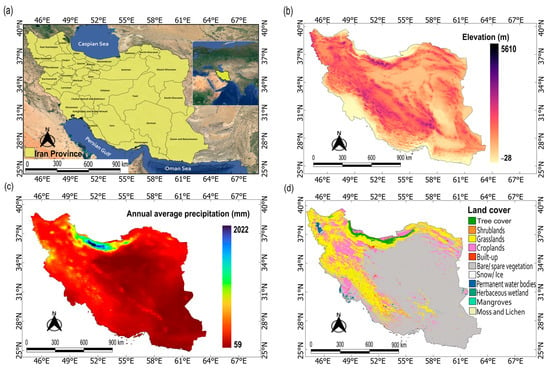
Figure 1
Figure 1
<p>Study area (Iran). Map showing (<b>a</b>) location of the study area(background Image is from Google Earth 2024 and the boundary data is from the Global Administrative Areas (GADM), <a href="http://www.gadm.org" target="_blank">http://www.gadm.org</a>, accessed on 12 May 2024), (<b>b</b>) topographic elevation of the study area (30 m digital elevation model data from United States Geological Survey (USGS)) [<a href="#B40-water-16-03334" class="html-bibr">40</a>], (<b>c</b>) mean annual precipitation between 2001 and 2022 based on precipitation data from Climate Hazards Group InfraRed Precipitation with Station Data (CHIRPS) [<a href="#B41-water-16-03334" class="html-bibr">41</a>], and (<b>d</b>) land cover map of the study area for the year 2021 adopted from the European Space Agency (ESA) [<a href="#B42-water-16-03334" class="html-bibr">42</a>].</p> Full article ">Figure 2
<p>Workflow of methodology for evaluating drought characteristics and impact on natural vegetation. SPEI was used during the growing season (October to April).</p> Full article ">Figure 3
<p>Spatial distribution of drought severity and frequency from 2001 to 2022 in Iran: (<b>a</b>) severity of drought events for all months; (<b>b</b>) severity of drought events in the growing season; (<b>c</b>) frequency of drought events for all months; and (<b>d</b>) frequency of drought events in the growing season.</p> Full article ">Figure 4
<p>Trends in drought severity per year in Iran from 2001 to 2022 based on the 1-month SPEI during the growing season (October to April). Panel (<b>a</b>) shows the magnitude and direction of the drought severity trend per year and panel (<b>b</b>) shows drought severity classes based on the direction of change (i.e., increasing, decreasing, or stable). Statistically insignificant (<span class="html-italic">p</span> > 0.05) changes (stable areas) are shaded in gray.</p> Full article ">Figure 5
<p>Spatial distribution of drought vegetation relationships across Iran. Panel (<b>a</b>) shows the correlation coefficient between NDVI anomaly and SPEI for five time scales (1, 3, 6, 9, and 12 months) without time lag (red: negative correlation, green: positive correlation), panel (<b>b</b>) shows a 1-month lag, and panel (<b>c</b>) shows a 2-month lag. Significant correlations (<span class="html-italic">p</span> < 0.05) during the growing season (October to April) across these time scales and lags are displayed, while non-significant correlations are masked. The dash vertical line shows the mean value.</p> Full article ">
Open AccessArticle
Morphometric Characterization and Dual Analysis for Flash Flood Hazard Assessment of Wadi Al-Lith Watershed, Saudi Arabia
by
Bashar Bashir and Abdullah Alsalman
Water 2024, 16(22), 3333; https://doi.org/10.3390/w16223333 - 20 Nov 2024
Abstract
Flash floods are one of the most hazardous natural events globally, characterized by their rapid onset and unpredictability, often overwhelming emergency preparedness and response systems. In the arid environment of Saudi Arabia, Wadi Al-Lith watershed is particularly prone to flash floods, exacerbated by
[...] Read more.
Flash floods are one of the most hazardous natural events globally, characterized by their rapid onset and unpredictability, often overwhelming emergency preparedness and response systems. In the arid environment of Saudi Arabia, Wadi Al-Lith watershed is particularly prone to flash floods, exacerbated by sudden storms and the region’s distinct topographical features. This study focuses on the morphometric characterization and comparative analysis of flash flood risk within the Wadi Al-Lith basin. To assess flood susceptibility, two widely adopted methodologies were employed: the morphometric ranking approach and El-Shamy’s method. A 12.5-m resolution ALOS PALSAR digital elevation model (DEM) was used to delineate the watershed and generate a detailed drainage network via Arc-Hydro tools in the ArcGIS 10.4 software. Fifteen morphometric parameters were analyzed to determine their influence on flood potential and hazard prioritization. The findings of this study provide crucial insights for regional flood risk management, offering an improved understanding of flash flood dynamics and assisting in developing effective mitigation strategies for Wadi Al-Lith and similar environments. The findings reveal that Wadi Al-Lith comprises multiple sub-catchments with varying degrees of vulnerability to flash flooding. According to the morphometric hazard analysis (MHA), certain sub-catchments, including sc-2, sc-4, sc-5, sc-6, sc-10, sc-12, sc-13, and sc-15, emerge as highly susceptible to flood hazards, while others (sc-1 and sc-9) fall into moderate risk categories. In contrast, the application of El-Shamy’s method provides a different ranking of flood risks across the watershed’s sub-catchments, offering a comparative view of flood susceptibility. The insights gained from this dual-analysis approach are expected to support the development of targeted flood prevention and mitigation strategies, which are essential for minimizing the future impacts of flash flooding in the Wadi Al-Lith watershed and ensuring better preparedness for local communities.
Full article
(This article belongs to the Special Issue Use of Remote Sensing Technologies for Water Resources Management)
►▼
Show Figures
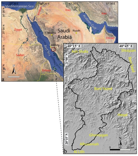
Figure 1
Figure 1
<p>(<b>a</b>) Regional map of Saudi Arabia and (<b>b</b>) hillshade map showing location of the Wadi Al-Lith watershed.</p> Full article ">Figure 2
<p>(<b>a</b>) A digital elevation model map and (<b>b</b>) the geomorphological zones of the Wadi Al-Lith watershed.</p> Full article ">Figure 3
<p>Chart illustrating the drainage systems and morphometric parameters analysis of the Wadi Al-Lith watershed.</p> Full article ">Figure 4
<p>(<b>a</b>) sub-catchments (1–15) and (<b>b</b>) different stream orders of the Wadi Al-Lith watershed.</p> Full article ">Figure 5
<p>Distribution of the morphometric parameter values for the 15 sub-catchments. Lb: basin length; Wb: basin width; Rlw: length width ratio; Os: stream order; Ns: stream number; Ls: stream length; Rb: bifurcation ratio; A: total area; P: perimeter; Re: elongation ratio; Rc: circulation ratio; sh-f: shape factor; Dd: drainage density; F: stream factor; Dt: stream texture.</p> Full article ">Figure 5 Cont.
<p>Distribution of the morphometric parameter values for the 15 sub-catchments. Lb: basin length; Wb: basin width; Rlw: length width ratio; Os: stream order; Ns: stream number; Ls: stream length; Rb: bifurcation ratio; A: total area; P: perimeter; Re: elongation ratio; Rc: circulation ratio; sh-f: shape factor; Dd: drainage density; F: stream factor; Dt: stream texture.</p> Full article ">Figure 6
<p>Flood susceptibility levels based on the ranking hazard approach.</p> Full article ">Figure 7
<p>El-Shamy method diagrams for assigning flash flood susceptibility classes. (<b>a</b>) Bifurcation ratio (Rb) against drainage density (Dd) and (<b>b</b>) bifurcation ratio (Rb) against stream frequency (Fs).</p> Full article ">Figure 8
<p>Flood susceptibility levels according to the El-Shamy method. (<b>a</b>) Rb ve Dd and (<b>b</b>) Rb ve Fs.</p> Full article ">
Open AccessArticle
Action of Low-Density Polyethylene Microspheres in the Transport of Metformin Hydrochloride in Aqueous Medium Through Adsorption and Desorption
by
Luanna Gláucia Guimarães, Renata Medici Frayne Cuba and Francisco Javier Cuba Teran
Water 2024, 16(22), 3332; https://doi.org/10.3390/w16223332 - 20 Nov 2024
Abstract
The present study addresses the issue of transporting pharmaceuticals via microplastics in aquatic environments. For this purpose, the adsorption and desorption of metformin hydrochloride (MET), a hydrophilic compound, on polyethylene microspheres (PMEs) were studied via batch adsorption and desorption capacity and kinetics tests.
[...] Read more.
The present study addresses the issue of transporting pharmaceuticals via microplastics in aquatic environments. For this purpose, the adsorption and desorption of metformin hydrochloride (MET), a hydrophilic compound, on polyethylene microspheres (PMEs) were studied via batch adsorption and desorption capacity and kinetics tests. The adsorption test results indicated minimal influence of pH values above 5, alongside a decrease in adsorption capacity with an increasing mass of PMEs. The Freundlich model best represented the adsorption capacity data; however, values of n < 1 (0.6) and low K suggest a decrease in the sorption affinity of MET with increasing initial MET concentration and a low affinity of MET for PM beads. The rate and equilibrium of adsorption were fast, and the results adequately fit the pseudo-first- and pseudo-second-order models, suggesting that physical and chemical mechanisms contributed to the adsorption of MET onto the PEMs under the conditions of this study. The desorption equilibrium result was 1.3 mg g−1 ± 0.04 mg g−1, without significant change, regardless of the initial amount of adsorbed MET. However, the desorption percentage varied between 26.14% and 7.01% as a function of the amount. of MET adsorbed onto the PMEs. These results suggest that PMEs could be potential vectors of MET transport in aquatic environments.
Full article
(This article belongs to the Special Issue Research on Water Supply Systems and on the Treatment and Recovery of Wastewater and Stormwater)
►▼
Show Figures
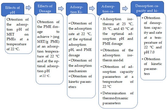
Figure 1
Figure 1
<p>Flowchart of the experimental approach.</p> Full article ">Figure 2
<p>Scanning electron microscopy images of PMEs used in this study. Magnification: (<b>a</b>) 90×, (<b>b</b>) 500×, (<b>c</b>) 1500×, and (<b>d</b>) 5000×. Arrows indicate the presence of cracks on the surface of the PMEs.</p> Full article ">Figure 3
<p>N<sub>2</sub> adsorption and desorption curves of the PMEs.</p> Full article ">Figure 4
<p>Illustration of the structure of the metformin molecule as a function of the pH of the medium [<a href="#B35-water-16-03332" class="html-bibr">35</a>]. Scheme 1—monoprotonated, Scheme 2—diprotonated, and Scheme 3—neutral.</p> Full article ">Figure 5
<p>MET adsorption capacity as a function of pH.</p> Full article ">Figure 6
<p>Adsorption capacity (q<sub>e</sub>) of MET as a function of the mass of PMEs.</p> Full article ">Figure 7
<p>Adsorption isotherms and data fit to the Freundlich model.</p> Full article ">Figure 8
<p>FTIR spectra of the PMEs before adsorption (PME) and after adsorption of metformin (PMES).</p> Full article ">Figure 9
<p>MET removal as a function of time.</p> Full article ">Figure 10
<p>Adsorption kinetics and data fit to the pseudo-first- and pseudo-second-order models.</p> Full article ">Figure 11
<p>Fitting data of MET adsorption onto PME spheres. Note: The assay was performed with an initial concentration of MET = 20 mg L<sup>−1</sup>, pH = 8.0, and temperature = 22 °C ± 1 °C.</p> Full article ">Figure 12
<p>Influence of temperature on MET adsorption onto PMEs.</p> Full article ">Figure 13
<p>Desorption capacity (q<sub>d</sub>) and efficiency (%) of the MET of the PMEs. Note: Assay conditions: 50 mL of regenerating solution (deionized water) with 6.0 < pH < 7.0. Temperature—22 °C.</p> Full article ">Figure 14
<p>Desorption kinetics. (<b>A</b>) Desorption capacity q<sub>td</sub> (mg g<sup>−1</sup>), and (<b>B</b>) % MET desorption. Note: 50 mL of deionized water, pH = 7.0, T = 22 °C, agitation = 100 rpm.</p> Full article ">
Open AccessArticle
Optimization of Real-Time Control Approach: Number, Placement, and Proportional–Integral–Derivative Control Rules of Flow Control Devices in Distributed Flood Routing
by
Hamidreza Jalili, Lizette Chevalier and John W. Nicklow
Water 2024, 16(22), 3331; https://doi.org/10.3390/w16223331 - 20 Nov 2024
Abstract
Climate change, through more frequent extreme weather events, and urban sprawl, by increasing runoff, are two critical threats to drainage networks, impacting both public health and property. Augmenting drainage networks to withstand additional stress by enlarging conduits or constructing new detention facilities requires
[...] Read more.
Climate change, through more frequent extreme weather events, and urban sprawl, by increasing runoff, are two critical threats to drainage networks, impacting both public health and property. Augmenting drainage networks to withstand additional stress by enlarging conduits or constructing new detention facilities requires a significant financial investment. The goal of this study is to enhance urban resilience by optimizing real-time control (RTC) systems for drainage networks that optimize the flow control devices (FCDs), which could mitigate the need to invest in major construction costs. RTC is an approach that can help mitigate flooding in urban areas. This study is the first to optimize feedback controllers in SWMM, as well as the first to simultaneously optimize the number, location, and proportional–integral–derivative (PID) controllers for FCDs through two nested genetic algorithms (GAs), and especially within a unified environment (i.e., Python), which led to more efficient management of the process, thereby enhancing the efficiency of urban drainage network optimization. This study examined the impact of optimized RTC on the urban drainage network (UDN) in a part of New Orleans, LA, USA, under 1-, 2-, 5-, and 10-year storm events. The optimized RTC resulted in an improvement of up to 50% in network performance during a design storm. The results demonstrate the applicability in an urban environment where storms, flooding, and financial investments are critical to the management of stormwater drainage.
Full article
(This article belongs to the Special Issue Advances in Water and Stormwater Networks: Modelling and Pollutant Degradation)
►▼
Show Figures
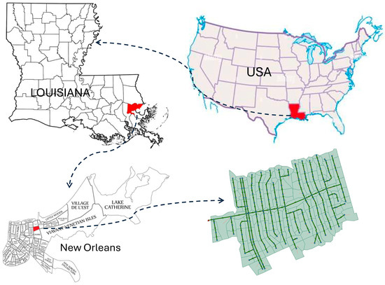
Figure 1
Figure 1
<p>Drainage network case study (New Orleans, LA, USA).</p> Full article ">Figure 2
<p>Locations of detention ponds in the existing drainage network that were removed.</p> Full article ">Figure 3
<p>IDF curves for New Orleans (PCSWMM).</p> Full article ">Figure 4
<p>Design storms with return periods of 1, 2, 5, and 10 years, and a rainfall duration of 30 min.</p> Full article ">Figure 5
<p>A schematic of the whole process.</p> Full article ">Figure 6
<p>Comparison of performance of the models with and without initial optimization.</p> Full article ">Figure 7
<p>Hydrographs at downstream conduit: comparison with and without RTC system for 30-min rainfall duration and 10-year return period.</p> Full article ">Figure 8
<p>Hydrographs at downstream end conduit: comparison with and without the RTC system for 30-min rainfall duration and 5-year return period.</p> Full article ">Figure 9
<p>Velocity vs. time at downstream conduit: comparison with and without the RTC system for 30-min rainfall duration and 5-year return period.</p> Full article ">Figure 10
<p>Depth vs. time at downstream conduit: comparison with and without the RTC system for 30-min rainfall duration and 5-year return period.</p> Full article ">Figure 11
<p>Hydrographs at downstream conduit: comparison with and without the RTC system for 30-min rainfall duration and 2-year return period.</p> Full article ">Figure 12
<p>Velocity vs. time at downstream conduit: comparison with and without the RTC system for 30-min rainfall duration and 2-year return period.</p> Full article ">Figure 13
<p>Depth vs. time at downstream conduit: comparison with and without the RTC system for 30-min rainfall duration and 2-year return period.</p> Full article ">Figure 14
<p>Hydrographs at downstream end conduit: comparison with and without the RTC system for 30-min rainfall duration and 1-year return period.</p> Full article ">Figure 15
<p>Velocity vs. time at downstream conduit: comparison with and without the RTC system for 30-min rainfall duration and 1-year return period.</p> Full article ">Figure 16
<p>Depth vs. time at downstream conduit: comparison with and without the RTC system for 30-min rainfall duration and 1-year return period.</p> Full article ">Figure 17
<p>Placement of the final orifices in the optimized RTC system; 2-Year return period.</p> Full article ">
Journal Menu
► ▼ Journal Menu-
- Water Home
- Aims & Scope
- Editorial Board
- Reviewer Board
- Topical Advisory Panel
- Instructions for Authors
- Special Issues
- Topics
- Sections & Collections
- Article Processing Charge
- Indexing & Archiving
- Editor’s Choice Articles
- Most Cited & Viewed
- Journal Statistics
- Journal History
- Journal Awards
- Society Collaborations
- Conferences
- Editorial Office
Journal Browser
► ▼ Journal BrowserHighly Accessed Articles
Latest Books
E-Mail Alert
News
Topics
Topic in
Molecules, Pollutants, Separations, Sustainability, Water
Sustainable Technologies for Water Purification
Topic Editors: Rakesh Govind, Barry T. HartDeadline: 30 November 2024
Topic in
Bioengineering, Catalysts, Processes, Sustainability, Water
Wastewater Treatment by Physical, Chemical, Photochemical, and Biological Processes, and Their Combinations
Topic Editors: Mehrab Mehrvar, Edgar Quiñones-Bolaños, Ciro Bustillo-Lecompte, Samira GhafooriDeadline: 31 December 2024
Topic in
Catalysts, Processes, Sci, Water, Sustainability
Advanced Oxidation Processes: Applications and Prospects, 2nd Volume
Topic Editors: Gassan Hodaifa, Antonio Zuorro, Joaquín R. Dominguez, Juan García Rodríguez, José A. Peres, Zacharias Frontistis, Mha AlbqmiDeadline: 31 January 2025
Topic in
Applied Sciences, Clean Technol., Energies, Membranes, Polymers, Sustainability, Water
New Advances in Membrane Technology and Its Contribution to Sustainability
Topic Editors: Patricia Luis Alconero, Bart Van der BruggenDeadline: 25 February 2025
Conferences
Special Issues
Special Issue in
Water
Application of Biochar in Wastewater Treatment and Purification
Guest Editors: Bing Wang, Masud HassanDeadline: 24 November 2024
Special Issue in
Water
More Holistic and Adaptive Decisions to Mitigate Climate Change Effects in Agricultural Water Resources Management
Guest Editor: Nektarios N. KourgialasDeadline: 25 November 2024
Special Issue in
Water
Hydrodynamics in Pressurized Pipe Systems
Guest Editor: Kamil UrbanowiczDeadline: 25 November 2024
Special Issue in
Water
Groundwater Depletion: Current Trends and Future Challenges to Mitigate the Phenomenon
Guest Editors: Nerantzis Kazakis, Micòl Mastrocicco, Konstantinos ChalikakisDeadline: 25 November 2024