Abstract
Although it is generally accepted that massive galaxies form in a two-phased fashion, beginning with a rapid mass buildup through intense starburst activities followed by primarily dry mergers that mainly deposit stellar mass at outskirts, the late time stellar mass growth of brightest cluster galaxies (BCGs), the most massive galaxies in the universe, is still not well understood. Several independent measurements have indicated a slower mass growth rate than predictions from theoretical models. We attempt to resolve the discrepancy by measuring the frequency of BCGs with multiple cores, which serve as a proxy of the merger rates in the central region and facilitate a more direct comparison with theoretical predictions. Using 79 BCGs at z = 0.06–0.15 with integral field spectroscopic data from the Mapping Nearby Galaxies at Apache Point Observatory (MaNGA) project, we obtain a multiple-core fraction of 0.11 ± 0.04 at z ≈ 0.1 within an 18 kpc radius from the center, which is comparable to the value of 0.08 ± 0.04 derived from mock observations of 218 simulated BCGs from the cosmological hydrodynamical simulation IllustrisTNG. We find that most cores that appear close to the BCGs from imaging data turn out to be physically associated systems. Anchoring on the similarity in the multiple-core frequency between the MaNGA and IllustrisTNG, we discuss the mass growth rate of BCGs over the past 4.5 Gyr.
Original content from this work may be used under the terms of the Creative Commons Attribution 4.0 licence. Any further distribution of this work must maintain attribution to the author(s) and the title of the work, journal citation and DOI.
1. Introduction
In the current cosmological paradigm, the mass content of the universe is dominated by cold dark matter (CDM), and expansion is governed by the so-called dark energy (which could take the form of a cosmological constant Λ). Structure formation proceeds in a bottom-up fashion; small dark matter halos form first, then grow by merging and accreting smaller halos (e.g., Peebles 1982; also see Baugh 2006 for a review). In modern theories of galaxy formation, galaxies are believed to form within dark matter halos (e.g., Rees & Ostriker 1977; White & Rees 1978; White & Frenk 1991). The dominant galaxy in a halo is often referred to as the central galaxy, and all other galaxies as satellites. As halos grow by mergers, their galaxy population grows correspondingly. Particularly, because of dynamical friction, massive galaxies from an infalling halo would typically sink quickly to the center of the larger halo and merge with the central galaxy, creating an even more massive galaxy, a process once called "galactic cannibalism" (Ostriker & Tremaine 1975). At the present time, the culmination of the hierarchical structure formation is clusters of galaxies, whose central galaxies are often known as "brightest cluster galaxies" (BCGs).
The growth paths BCGs experience potentially contains important constraints on cluster and galaxy formation. BCGs are usually found at or near the center in their host cluster (e.g., Lin & Mohr 2004). It is observed that the Ks -band luminosity or stellar mass of BCG show a correlation with the mass and velocity dispersion of its host cluster (e.g., Lin & Mohr 2004; Whiley et al. 2008; Lidman et al. 2012; Kravtsov et al. 2018; Golden-Marx et al. 2021). Furthermore, the extended stellar envelop of BCGs could potentially serve as a better proxy of the cluster halo mass than richness (Huang et al. 2021).
A variety of evidence points to the special status of BCGs among cluster member galaxies. Because of its central location within the host cluster, galactic cannibalism inevitably takes place. The tidal debris stripped from cluster galaxies contributes to the light of central galaxies (Richstone 1976). In addition, BCGs are found to form a separate population, distinctive with respect to the extreme of the cluster galaxy luminosity/stellar mass function (Tremaine & Richstone 1977; Lin et al. 2010; Rong et al. 2018; Dalal et al. 2021). Moreover, the major axis of BCGs are found to often align with the cluster orientation (Sastry 1968; Niederste-Ostholt et al. 2010).
Recent numerical simulations and semi-analytical models (SAMs) suggest that massive galaxies, BCGs included, form in a two-phase scenario. Stars form intensely in the progenitors at high redshifts, and late time (z < 1) assembly is dominated by dissipationless mergers (e.g., De Lucia & Blaizot 2007; Oser et al. 2010; Laporte et al. 2013; Rodriguez-Gomez et al. 2016; Ragone-Figueroa et al. 2018; Jing et al. 2021). However, there appears to be a discrepancy in BCG stellar mass growth between model predictions and observations. Lin et al. (2013) find good agreement in the mass growth history between observations and model prediction at z = 0.5–1.5; however, there seems to be a halt in the growth of real BCGs at z < 0.5, while model BCGs continue to grow. Inagaki et al. (2015) investigate the mass growth in BCG at z < 0.5, using the so-called "top-N" method (that is, selecting the top N most massive clusters in a given comoving volume over different cosmic epochs), and conclude from observations that the mass growth is less than 14% between z = 0.4 and 0.2, while the SAM of Guo et al. (2011) predicts at least 30%. Similarly, Lidman et al. (2012) find a factor of 1.5 times smaller mass growth at z = 0.3–1 compared to the simulation prediction (see also Zhang et al. 2016). A recent work by Lin et al. (2017), using deep photometry from the Subaru Hyper Suprime-Cam Survey (Aihara et al. 2018), shows that BCGs typically grow by about 35% between z = 1 and z = 0.3 (again using the top-N approach), while the SAM of Guo et al. (2013) suggests a factor of 2 larger growth rate.
Such a discrepancy could be explained if, for mergers occurring at late times, BCGs mainly accrete mass into their extended outskirts, beyond the observational photometry apertures (Whiley et al. 2008; Inagaki et al. 2015). Ragone-Figueroa et al. (2018) analyze hydrodynamical simulations and obtain a smaller stellar mass growth factor that is consistent with observations by using an aperture similar to that of observations (30 and 50 kpc). This result suggests that a more direct comparison between observation and simulation is required to solve this discrepancy. However, it is difficult to measure the total luminosity of BCGs, which often have extended surface brightness profiles in the crowded cluster regions. It requires not only deep imaging data with a flattened sky and very careful treatments of background subtraction and source masking, but also sophisticated modeling techniques (e.g., Huang et al. 2013, 2016, 2018; Meert et al. 2013, 2016; Fischer et al. 2019; Wang et al. 2021).
Another approach to this problem is to measure the merger rate of BCGs close to their centers. The N-body simulations of Gao et al. (2004) suggest that BCGs have gone through many merging events that bring material to the innermost region of ∼10 kpc, even at z < 1. This implies that these mergers, corresponding to the "second phase" in the two-phase scenario mentioned above, not only affect the outskirts of the BCGs, but also have strongly observable effects in the central region.
One can define the merger rate as the probability of a BCG with two or more closely separated cores to be observed per unit time:

which is the combination of the "multiple-core frequency" with a merger timescale, which we term the "visibility time" here. Very close pairs are also called multiple nuclei or multiple cores, because the secondary/satellite galaxies, during the merger process with a BCG, often appear as an additional core of the BCG (Schneider et al. 1983; Lauer 1988). We use the term "multiple-core frequency" fmc for the fraction of BCGs that appear as multiple-cored in a volume-limited sample. The visibility time, defined to be the duration for a satellite to remain "visible" (i.e., identifiable from imaging or spectroscopy) during the course of galactic cannibalism, has to be derived from numerical simulations, or estimated from theory. On the other hand, the multiple-core frequency is an observable that provides the opportunity for a direct comparison between observations and models. The same quantity for pairs with larger separation (e.g., when the two galaxies are clearly seem as separate entities) is often named "pair fraction" in the literature (e.g., McIntosh et al. 2008; Liu et al. 2009; Groenewald et al. 2017).
The pair fraction as a critical step toward deriving merger rates of central galaxies in massive halos such as groups and clusters has been widely used (e.g., Edwards & Patton 2012; Burke & Collins 2013; Lidman et al. 2013). While morphological distortions of galaxies in a pair can be an indication of interaction, thus serving as an (indirect) indicator of physical association of the pair (Lauer 1988; McIntosh et al. 2008; Liu et al. 2009, 2015), the most reliable way to identify pairs is through spectroscopy (e.g., Groenewald et al. 2017). Brough et al. (2011) and Jimmy et al. (2013) conduct the first targeted integral field spectroscopy (IFS) observation of BCGs with close companions.
In this work, we present a measurement of multiple-core frequency of the largest sample of BCGs to date, using IFS data from the Mapping Nearby Galaxies at Apache Point Observatory (MaNGA; Bundy et al. 2015; Drory et al. 2015; Law et al. 2015, 2016, 2021; Yan et al. 2016a, 2016b) project, which is part of the fourth generation of the Sloan Digital Sky Survey (SDSS-IV; Gunn et al. 2006; Smee et al. 2013; Blanton et al. 2017). We further compare our measurement with results from the cosmological hydrodynamical simulation IllustrisTNG (Weinberger et al. 2017; Marinacci et al. 2018; Naiman et al. 2018; Nelson et al. 2018, 2019; Pillepich et al. 2018a, 2018b; Springel et al. 2018) to examine the consistency between observations and models.
This paper is structured as follows. In Section 2, we present the essential ingredients of our analysis, including the cluster sample, the imaging and IFS data, and the simulation. In Section 3, we describe in detail our method for extracting the multiple-core frequency from core detection in images to confirmation of physical association using MaNGA velocity maps. We carry out a similar analysis on mock images of simulated BCGs in Section 4. We compare our results with some of the findings from the literature in Section 5, where we also show that the BCG samples used in our analysis are unbiased with respect to the general BCG population. We conclude in Section 6. In Appendix A, we present a comparison of several kinds of photometric measurements used in our analysis, showing consistency among them. In Appendix B, we describe BCGs that either require special treatment for their photometry, or have to be excluded due to various reasons.
We adopt a cosmology with a Hubble constant of H0 = 100 h km s−1 Mpc−1, with h = 0.73, ΩM = 0.27, and ΩΛ = 0.73 throughout this paper. We use halo mass defined as M180m in observations and M200m in the simulation. These corresponds to the mass contained within a radius R180m (R200m ) within which the mean density is 180 (200) times the mean density of the universe. The difference between M180m and M200m is within 2% so the two can be approximated as the same quantity.
2. Elements of Analysis
2.1. The MaNGA BCG Sample
MaNGA has obtained spatially resolved spectroscopy for about 10,000 galaxies out to z = 0.15. The data are obtained by integral field units (IFUs) built with fiber bundles, which have diameters ranging from 12'' to 32'', providing a spatial sampling 1–2 kpc (at the typical redshift of MaNGA galaxies, z ≈ 0.03). The MaNGA sample is constructed to have a flat stellar mass distribution, and consists of the primary, secondary, color-enhanced, and ancillary samples (Wake et al. 2017). The primary sample has their IFU coverage to 1.5 times the effective radius (Re ) and the secondary to 2.5 Re . The ancillary programs focus on special types of galaxies such as massive galaxies, merger candidates, and active galaxies. In particular, the "BCG" ancillary program has enabled comprehensive studies of the kinematic morphology–density relation and the angular momentum content of massive central galaxies (Greene et al. 2017, 2018).
Our parent BCG sample is taken from the group and cluster catalog of Yang et al. (2007, hereafter Y07), updated to the version based on SDSS data release 7 (DR7; Abazajian et al. 2009). Among the three versions of catalogs provided, we adopt the one that is constructed using the SDSS model magnitude 22 and includes additional redshifts from the literature, in order to have the largest number of clusters. We apply a cut in the cluster mass M180m ≥ 1014 h−1 M⊙, which results in 4033 clusters. We note in passing that the halo mass provided by Y07 is estimated by the ranking of total stellar mass of a cluster/group.
The details of BCG selection are described in Yang et al. (2005, see Section 3.2 therein). Note that the BCG is the most luminous galaxy among the members and may not necessarily be close to the cluster center (e.g., Skibba et al. 2011), which is the geometric and luminosity-weighted center of member galaxies. Matching the 4033 BCGs with the 8113 galaxies released from MaNGA Product Launch-9 (MPL-9), we obtain 128 BCGs. These galaxies belong to the MaNGA primary, secondary, and color-enhanced sample, as well as the "BCG" and "MASSIVE" ancillary programs (Wake et al. 2017). The 128 clusters lie at z = 0.02–0.15, and are all detected in the X-rays by Wang et al. (2014). Hereafter we shall refer to this sample as "MPL-9 BCGs" (see Tables 1 and 2).
Table 1. Definition of BCG Samples
| Name | Number | Definition |
|---|---|---|
| All | 4033 | All of Y07 clusters with M180m ≥ 1014 h−1 M⊙ (Section 2.1) |
| MPL-9 | 128 | "All" matched to MaNGA MPL-9 (Section 2.1) |
| Main | 79 | "MPL-9" with problematic BCGs removed and having IFU coverage to ≥18 kpc (Section 3.2) |
| Volume-limited | 73 | Same as "Main," but with stellar mass above stellar completeness limit (Equation (3); Section 3.6) |
| Parent | 1359 | Same as "All," but above the completeness limit and at z = 0.02–0.15 (Section 3.6) |
| TNG-Comparison | 225 | Similar to Parent, but at z = 0.07–0.11 and within a volume of (300 Mpc)3 (Section 4.1) |
| Not-in-MaNGA | 1237 | Same as "Parent," but excluding the MPL-9 sample (Section 5.1.1) |
Download table as: ASCIITypeset image
The algorithm used in the cluster finder of Yang et al. (2005) selects the BCG solely based on the luminosity. However, sometimes the brightest galaxy in a cluster has a spiral morphology. Given that it is unlikely for a central galaxy of a virialized, matured cluster to be a spiral (Coziol et al. 2009), we decide to visually inspect all MPL-9 BCGs using images from the SDSS, with the aid of the g − r versus i color–magnitude diagrams of cluster members (see, e.g., Figure 27 for examples). In this paper, we regard BCGs to be of early type morphology 23 and also the most luminous galaxies in each cluster. If the BCG candidates show a spiral morphology (which makes it quite difficult for the detection of multiple cores given our methodology as described below; in total five spiral BCG candidates are discarded), or are not the brightest galaxy on the red sequence, we search for other possible candidates. If there is no better candidate, or the better candidate is not observed by MaNGA, we remove the cluster from the sample. Six clusters are removed due to the above reasons (please see Appendices B.3 and B.4.1 for more details). The Coma cluster is also removed because it does not have the same type of data products as other BCGs in our sample. Therefore, we obtain 121 visually confirmed BCGs. We emphasize that our BCG selection is primarily that of Y07; only 5 of the 128 galaxies initially defined as BCGS were redefined through visual inspection (see Appendices B.3 and B.4.1). Our main conclusion is not affected by redefining these 5 BCGs.
In addition, there are 6 BCGs with nearby bright stars, or are severely affected by the edges of mosaic frames that would make their photometry unreliable (see Section 3.1). As these events are independent of the multiple-core frequency, these BCGs are also removed from our analysis (see Appendix B.4.2). There are 115 BCGs left after these cuts.
2.2. The BCG Sample from IllustrisTNG
IllustrisTNG is a series of cosmological hydrodynamical simulations that has three simulation volumes, TNG50, TNG100, and TNG300. We use the simulation TNG300-1 (hereafter simply TNG300), which has a box size of 300 Mpc on a side, to maximize our sample size of simulated BCGs. TNG300-1 has 2 × 25003 resolution elements, and a mass resolution of 1.1 × 10⁷ M⊙ for baryons and 5.9 × 10⁷ M⊙ for dark matter. The gravitational softening length (for stars and dark matter) of 1.5 kpc at z = 0.
The average redshift of our MPL-9 sample of 128 BCGs is z = 0.1. Therefore, we select BCGs from snapshot 91 of TNG300, which corresponds to z = 0.0994. There are 225 halos with mass M200m ≥ 1014 h−1 M⊙ identified using the friends-of-friends (FoF) algorithm (Davis et al. 1985). The main subhalos of these halos are identified as the BCGs (via the SUBFIND algorithm; Springel et al. 2001). In Section 4, we will describe our methods to mimic the selection of BCGs as closely as possible to our MaNGA sample, and how we derive multiple-core frequency from synthetic images of the resulting BCG sample.
3. An IFU Survey of Multiple-core Frequency of Brightest Cluster Galaxies
Our analysis consists of four steps: (1) modeling the light distribution of a BCG using SDSS imaging data; (2) subtracting the best model of the BCG from the image and measuring the position and fluxes of the core(s), if present; (3) finding the counterpart(s) of the core(s) in the MaNGA stellar velocity map, and determining whether the core(s) are physically associated with the BCG; and (4) estimating the core-to-BCG flux ratio. Furthermore, we need to examine the completeness of our BCG selection, and apply correction factors where needed. We describe each of these steps in detail in the following.
Although in Equation (1) it is implied that the multiple-core frequency is simply the number of BCGs with multiple cores (NBCG, mc) divided by the total number of BCGs in a complete sample (NBCG), in reality, there are often cases where more than one satellite is merging with a BCG (i.e., there will be >1 cores). Given that each merger event should be independent, we thus define formally the multiple-core frequency fmc to be

where the numerator on the right denotes the total number of cores, instead of the number of BCGs with multiple cores.
3.1. Photometry of BCGs
The BCG photometry is somewhat ill-defined for several reasons. First, the surface brightness profiles of elliptical galaxies can usually be described by a Sérsic (Sérsic 1963) profile with an index n ≳ 3 or so (e.g., Kormendy et al. 2009), and such profiles, as well as actual observations, do not exhibit a well-defined/sharp edge. Moreover, as BCGs are very spatially extended, with a substantial fraction of their flux below the sky level, we can only extrapolate the profile we assumed to obtain the flux in this unconstrained region. Second, BCGs have much more complex profiles than common ellipticals, and it may require >2 Sérsic components to describe their surface brightness profiles. The properties such as position angle or color of the inner to outer region of BCGs can be quite different (Huang et al. 2013, 2016). Third, BCGs are often located in crowded regions. Cluster members surround, touch, or merge with BCGs, making it difficult to mask them out or deblend them from BCGs without affecting the photometric measurement. These all add to the uncertainty in the photometry of BCGs. Below we discuss how we obtain BCG photometry that is reliable enough for our needs.
We have two ways of obtaining the photometric measurements, such as Re and total magnitude. Our primary resources are the photometric catalogs of Meert et al. (2016, hereafter M16) and Fischer et al. (2019, hereafter F19). These catalogs are generated by the 2D fitting pipeline PyMorph (Meert et al. 2013, 2015) that uses GALFIT (Peng et al. 2002) as the engine for galaxy morphology modeling, and have a better estimation of the brightness than the SDSS pipeline for the most luminous galaxies, because of better sky subtraction, as well as more flexible modeling (two Sérsic components; Bernardi et al. 2017). We use the "Best model" table of M16 and remove the galaxies flagged as bad (flag = 20). For the BCGs that do not have a good fit in M16, we use the F19 catalog. F19 mark the preferred model for each galaxy with the "FLAG_FIT" flag; if there is no preference, we use the Sérsic+Exponential model. 74 out of our 115 BCGs have reliable magnitude and Re measurements from these two catalogs.
For BCGs not included in either of the catalogs of M16 or F19, we obtain their total magnitudes by running the code Ellipse on SDSS mosaic images (see below). Ellipse is a fully automated Python package for fitting ellipses to isophotal contours of galaxies, developed by Dr. G. Torrealba. 24 As a consistency check, we fit a single Sérsic profile to the surface brightness measured by Ellipse and find good agreement in the total flux with M16 and F19 catalogs (please see Appendix A for more details).
The images of BCGs are taken from SDSS DR12 (Alam et al. 2015). Our BCG sample has a typical Re of 10'' at its mean redshift of 0.1. Given the size of the BCGs, we need to have a large enough area to capture the extended profile and successfully perform sky subtraction. As BCGs often do not lie within one single "corrected frame" of the SDSS, we need to construct mosaic'd images, which are obtained from the SDSS DR12 Science Archive Server (SAS) as well as through the URL tool of DESI Legacy Imaging Survey 25 (Dey et al. 2019). We have confirmed that the images obtained from the two methods are identical. In practice, we use the URL tool of the DESI Legacy Imaging Survey because the SDSS SAS does not support bulk downloads. We use the i-band images for modeling the BCGs, because they show the multiple-core features most clearly, and some cores are only distinguishable from the BCG in the i band.
3.2. Maximum Projected Distance and IFU Coverage for Core Detection
As we want to focus on mergers taking place in the central parts of BCGs, we need to define a maximum distance (from the BCG center) for our search of secondary cores. There are two factors in our consideration for the maximum distance. The first one is the aperture size of the IFUs, as it directly limits the maximum separation of multiple cores practically. The second one is whether to have the distance defined to be a certain fraction of Re . We choose to use a fixed metric distance, so that a direct comparison can be made when applying our procedures to mock images of simulated BCGs (see Section 4.4).
The median Re of the 74 BCGs with photometric measurements from M16 and F19 is 17.5 kpc. Balancing between the IFU coverage and the maximum projected distance, we decide to select the BCGs that are covered by their IFU to at least 18 kpc, in order to have the largest sample size (which effectively also sets a lower redshift limit in our sample at z ≈ 0.06). Our final sample consists of 79 BCGs, which shall be referred to as the "Main" sample (Table 1).
3.3. Identifying Multiple Cores in SDSS Images
After downloading the SDSS mosaics, the images are cropped to sizes between 500 × 500 pixels and 1818 × 1818 pixels (6' × 6') for further analyses. We focus on the profile within 150 kpc, which corresponds to an image size of 682 pixels for the most nearby BCG in our sample. We also generate axisymmetric galaxy models with GALFIT to examine the effect of limited image size on the recovery of Re and total flux. For galaxy models with Re in the range of 10–40 pixels and with Sérsic indexes between 1 and 8, results from our tests suggest that images of 800 × 800 pixels can result in 78%–100% of the true Re . Hence image sizes larger than 800 pixels on a side would serve our goals well.
We feed these images cutouts to the source extraction software SExtractor (Bertin & Arnouts 1996) to obtain their segmentation maps. By varying parameters such as BACK_SIZE (controlling the size of the grid of background measurement), the way weight maps are obtained (either supplied by the SDSS or generated by SExtractor), and the sizes of input images, we find that the resulting maps do not sensitively depend on these choices. Small differences occur occasionally on some images with very bright stars or very crowded regions. We mainly use the 800 × 800 pixel images and set BACK_SIZE = 160 (that is, 1/5 of the image size). In 4 cases (out of 89), we need to resort to 1000 × 1000 pixel images in order to obtain a reasonable segmentation map.
To detect the cores in the images, we need to remove the light of the main body of the BCGs. We subtract the SExtractor measured background from the images, masked out the segmentation region of the sources touching the BCGs, and substitute the masked regions that are not connected to the BCG with a Gaussian noise that has the same standard deviation as the sky measured by SExtractor. These images, now with the BCG left as the only source, are then fed to Ellipse, which outputs empirical surface brightness models and profiles (in a similar fashion to the "ellipse" task in IRAF; Jedrzejewski 1987). We subtract the empirical models from the image to obtain the "BCG-free" residual maps. An example of an image, the model, and a residual map is shown in the upper row of Figure 1.
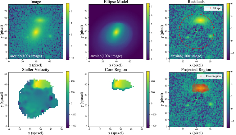
Figure 1. Demonstration of the procedure of core detection, using BCG No. 6 in our sample as an example. The upper row shows the SDSS i-band image of BCG No. 6, the model produced by Ellipse, and the residual map. These three images are displayed in the stretching of arcsinh(100×), and zoomed in to the central 80 pixels. The values shown on the color bars correspond to arcsinh(100× flux/nanomaggy), a convention used in all such SDSS (or mock SDSS) images throughout the paper. The red circle of 18 kpc from the BCG center is plotted on the residual map. The pixel scale of the SDSS images is 0396 pixel−1. The lower row shows the stellar velocity map with systemic velocity corrected (if needed), the detected core segmentation region, and the position of the core segmentation spaxels over the residual map. Note that the two rows are not plotted in the exact same scale.
Download figure:
Standard image High-resolution imageOn the residual maps, we run the Python implementation of SExtractor, SEP (Barbary 2016), with strong deblending parameters 26 and a low detection threshold to detect any possible core with 1.8–18 kpc separation from the BCG center. The lower limit, 1.8 kpc, is set to avoid identifying residuals of the BCG main body due to imperfections in the model as spurious cores; such cases, if present, will be safeguarded by our next step (kinematic confirmation via MaNGA velocity maps) as well as our final visual inspection. In addition, such a lower limit can avoid the blurring of images due to seeing. The upper-right panel of Figure 1 shows the 18 kpc circle and a detected core.
3.4. Identifying True Merging Systems with MaNGA Velocity Maps
To distinguish the merging systems from chance projections, we make use of the Python package Marvin (Cherinka et al. 2019), specifically designed to display and conduct calculations with various IFU maps produced by the MaNGA Data Analysis Pipeline (DAP; Belfiore et al. 2019; Westfall et al. 2019). We apply the DAP "DONOTUSE" mask to the maps to avoid spaxels that are not suitable for scientific analyses.
Subsequently, we need to remove any contribution from the systemic velocity of the galaxy. The MaNGA stellar velocity maps are corrected to the redshift from the NASA-Sloan Atlas 27 (NSA) catalog if available; otherwise the redshift is estimated by the DAP. However, sometimes, especially for complex galaxies that have multiple cores (or a fiber bundle containing foreground/background objects), the redshift can be inaccurate, or is not corrected to the object we identify as the main body of the BCG. We deal with this issue through the following steps. We first take the minimum absolute value between the value of central spaxel and the median value of the spaxels with signal-to-noise ratios (S/Ns) larger than 10. If this absolute value is ≤50 km s−1, we regard this object to have a reasonable redshift measurement. If the absolute value is >50 km s−1, the redshift may be problematic and requires correction. We set the new reference point at the median velocity of spaxels with S/N > 10. This definition avoids contamination from the cores in the central region. We apply the equation in Section 7.1.4 in Westfall et al. (2019) to correct the velocity map relative to the new reference point. These corrected maps are used to calculate the velocity offset between the cores and the BCG. For BCGs with rotation features, these features might be detected as a large core by our extraction pipeline, however. Therefore, we manually select the velocity maps with strong rotation features, fit a 3D plane to it, and subtract the velocity structure of that plane. We only use these subtracted maps in the extraction process, and do not use them when calculating the velocity offsets of the cores. The BCGs with strong rotation features are Nos. 6, 25, 26, 39, 51, 102, 107, 116, 117, 124 (Table 2).
Table 2. The 128 BCGs in the MPL-9 Sample
| ID | R.A. | Decl. | z (Y07) |

| Plateifu | Selected | Phot | IFU18kpc |
|---|---|---|---|---|---|---|---|---|
| 1 | 213.834862 | 52.3459366 | 0.0745125 | 14.00 | 8591-3704 | 1 | 1 | 0 |
| 2 | 195.088192 | 26.7887007 | 0.1460274 | 14.00 | 11009-6104 | 1 | 1 | 1 |
| 3 | 119.023042 | 33.7445348 | 0.0742991 | 14.01 | 8977-3703 | 1 | 1 | 0 |
| 4 | 126.502387 | 40.9811098 | 0.0575645 | 14.01 | 10496-6104 | 1 | 0 | 0 |
| 5 | 249.101963 | 28.6177833 | 0.1444254 | 14.02 | 11823-12704 | 1 | 1 | 1 |
| 6 | 131.301993 | 29.3062335 | 0.0999816 | 14.02 | 10499-6101 | 1 | 1 | 1 |
| 7 | 132.787323 | 27.355888 | 0.1198074 | 14.02 | 9506-6103 | 1 | 2 | 1 |
| 8 | 248.02191 | 13.6474084 | 0.0522497 | 14.02 | 8609-9102 | 1 | 0 | 0 |
| 9 | 177.546947 | 53.7225048 | 0.060313 | 14.02 | 11872-12701 | 1 | 1 | 0 |
| 10 | 127.528158 | 45.3517744 | 0.1482441 | 14.03 | 8725-6104 | 1 | 2 | 1 |
| 11 | 240.348548 | 26.1161536 | 0.0875589 | 14.03 | 9089-6103 | 1 | 0 | 0 |
| 12 | 118.11363 | 19.5401717 | 0.1155163 | 14.03 | 9497-6101 | 1 | 2 | 1 |
| 13 | 222.810125 | 32.3782013 | 0.0883005 | 14.03 | 9002-3703 | 1 | 2 | 0 |
| 14 | 235.475817 | 28.1340056 | 0.03322 | 14.03 | 9888-12701 | 0 | 2 | 0 |
| 15 | 247.694963 | 47.7948292 | 0.1279589 | 14.03 | 8483-6104 | 0 | 0 | 0 |
| 16 | 212.955985 | 52.8167901 | 0.076489 | 14.04 | 8591-6102 | 1 | 1 | 0 |
| 17 | 168.743724 | 53.6250028 | 0.1048493 | 14.04 | 9000-9101 | 1 | 1 | 1 |
| 18 | 181.827567 | 46.7275499 | 0.1014518 | 14.04 | 8261-3702 | 1 | 0 | 0 |
| 19 | 258.84568 | 57.4112548 | 0.0273026 | 14.05 | 8625-12704 | 1 | 2 | 0 |
| 20 | 229.429418 | 27.8953518 | 0.1195061 | 14.05 | 9891-12701 | 1 | 2 | 1 |
| 21 | 148.962806 | 1.57813456 | 0.100966 | 14.05 | 10845-3701 | 1 | 1 | 0 |
| 22 | 213.970379 | 50.323853 | 0.0738916 | 14.06 | 9864-12702 | 1 | 2 | 1 |
| 23 | 163.03258 | 44.77343 | 0.1395 | 14.06 | N/A | 0 | 0 | 0 |
| 24 | 119.617129 | 37.7866182 | 0.042836 | 14.07 | 9181-12702 | 1 | 2 | 0 |
| 25 | 122.867045 | 43.6383289 | 0.1429993 | 14.08 | 10213-3701 | 1 | 1 | 1 |
| 26 | 121.449567 | 25.2566188 | 0.1408135 | 14.08 | 9503-3703 | 1 | 0 | 1 |
| 27 | 48.5733376 | −0.6096748 | 0.1152619 | 14.08 | 8081-3701 | 1 | 2 | 0 |
| 28 | 215.964753 | 40.258839 | 0.0821963 | 14.08 | 8335-6103 | 1 | 1 | 0 |
| 29 | 139.94524 | 33.7497418 | 0.0229126 | 14.08 | 10505-6102 | 1 | 0 | 0 |
| 30 | 246.426331 | 43.9317681 | 0.1331387 | 14.09 | 8555-3702 | 1 | 1 | 1 |
| 31 | 122.615469 | 40.4306353 | 0.0982483 | 14.09 | 9486-6103 | 1 | 2 | 1 |
| 32 | 206.209062 | 52.7760145 | 0.1398773 | 14.09 | 9884-6102 | 1 | 1 | 1 |
| 33 | 225.682826 | 53.046861 | 0.1338617 | 14.09 | 8593-3701 | 1 | 0 | 1 |
| 34 | 228.451854 | 28.0329749 | 0.114432 | 14.10 | 9891-3701 | 1 | 2 | 0 |
| 35 | 122.18108 | 14.7892 | 0.08554 | 14.10 | N/A | 0 | 0 | 0 |
| 36 | 234.16229 | 25.9068083 | 0.0946412 | 14.11 | 9889-3703 | 1 | 0 | 0 |
| 37 | 46.49724 | −0.16648 | 0.10705 | 14.11 | 9194-9101 | 0 | 0 | 1 |
| 38 | 122.560974 | 20.2072517 | 0.1247102 | 14.11 | 9490-9102 | 1 | 1 | 1 |
| 39 | 225.62102 | 52.7339826 | 0.133075 | 14.12 | 8593-3704 | 1 | 1 | 1 |
| 40 | 244.683117 | 25.9474202 | 0.14518 | 14.12 | 9046-6102 | 1 | 0 | 1 |
| 41 | 137.141134 | 16.0465505 | 0.0719147 | 14.12 | 8248-6101 | 1 | 1 | 0 |
| 42 | 157.650761 | 35.9166146 | 0.1235215 | 14.12 | 8943-3704 | 1 | 1 | 1 |
| 43 | 121.603933 | 17.4177001 | 0.1041438 | 14.13 | 10497-12702 | 1 | 1 | 1 |
| 44 | 247.724345 | 24.5620962 | 0.0632161 | 14.13 | 9892-3701 | 1 | 0 | 0 |
| 45 | 146.523062 | 34.6242592 | 0.1342496 | 14.13 | 10838-12702 | 1 | 0 | 1 |
| 46 | 322.115223 | 0.18204297 | 0.1382348 | 14.13 | 8616-3702 | 1 | 1 | 1 |
| 47 | 168.406003 | 47.4871527 | 0.1120715 | 14.14 | 10509-12704 | 1 | 0 | 1 |
| 48 | 137.44131 | 41.9558691 | 0.1400345 | 14.14 | 8247-9102 | 1 | 1 | 1 |
| 49 | 238.299753 | 27.5557304 | 0.1474349 | 14.14 | 9888-6104 | 1 | 1 | 1 |
| 50 | 60.0838005 | −5.5852549 | 0.1308573 | 14.14 | 8728-3703 | 1 | 2 | 1 |
| 51 | 241.840776 | 28.8516181 | 0.126337 | 14.15 | 9030-9101 | 1 | 0 | 1 |
| 52 | 175.54471 | 55.45825 | 0.13339 | 14.15 | 8995-6103 | 1 | 1 | 1 |
| 53 | 125.388172 | 55.1520274 | 0.0796762 | 14.17 | 10494-12704 | 1 | 0 | 1 |
| 54 | 227.041415 | 29.2222 | 0.1109796 | 14.17 | 9891-9101 | 1 | 2 | 1 |
| 55 | 204.112347 | 54.8983344 | 0.1067703 | 14.17 | 11020-12702 | 1 | 1 | 1 |
| 56 | 127.105745 | 24.6230533 | 0.0883995 | 14.18 | 8939-6104 | 1 | 2 | 0 |
| 57 | 117.48113 | 29.4201944 | 0.0623623 | 14.18 | 8146-12704 | 1 | 0 | 1 |
| 58 | 157.921418 | 36.0233668 | 0.0852559 | 14.19 | 8943-9102 | 0 | 2 | 1 |
| 59 | 157.723276 | 41.2211227 | 0.092116 | 14.19 | 8455-12703 | 1 | 1 | 1 |
| 60 | 183.997375 | 35.7173765 | 0.1333452 | 14.19 | 8554-6103 | 1 | 2 | 1 |
| 61 | 131.63527 | 29.5987137 | 0.0701255 | 14.20 | 10499-12702 | 1 | 0 | 1 |
| 62 | 209.18658 | 44.90331 | 0.12504 | 14.21 | 8328-3703 | 1 | 0 | 1 |
| 63 | 252.565435 | 23.5798277 | 0.0360614 | 14.21 | 11979-12701 | 0 | 0 | 0 |
| 64 | 181.368271 | 51.4799899 | 0.0853738 | 14.21 | 10508-6102 | 1 | 1 | 0 |
| 65 | 255.471297 | 35.0510989 | 0.108797 | 14.21 | 8614-12701 | 1 | 0 | 1 |
| 66 | 240.832659 | 25.453721 | 0.0895342 | 14.24 | 9092-12704 | 1 | 0 | 1 |
| 67 | 312.909237 | −0.0558668 | 0.107683 | 14.25 | 9191-6103 | 1 | 0 | 1 |
| 68 | 205.6749428 | 26.23977838 | 0.065362 | 14.25 | 8983-12703 | 1 | 2 | 1 |
| 69 | 118.36082 | 29.3594463 | 0.0605648 | 14.26 | 8937-12705 | 1 | 2 | 0 |
| 70 | 254.933112 | 32.6153255 | 0.1013 | 14.26 | 9883-9101 | 1 | 2 | 1 |
| 71 | 241.877644 | 23.2363 | 0.0894408 | 14.26 | 9087-6102 | 1 | 0 | 0 |
| 72 | 246.172233 | 25.3282368 | 0.1284911 | 14.27 | 9048-3703 | 1 | 2 | 1 |
| 73 | 232.542819 | 29.0083925 | 0.0841925 | 14.27 | 9042-3702 | 1 | 2 | 0 |
| 74 | 169.669505 | 45.5527444 | 0.1126036 | 14.27 | 8466-6104 | 1 | 2 | 1 |
| 75 | 220.178483 | 3.46542146 | 0.0273424 | 14.27 | 11835-9101 | 0 | 0 | 0 |
| 76 | 129.372907 | 43.8693671 | 0.1354883 | 14.28 | 11745-9102 | 1 | 0 | 1 |
| 77 | 219.437785 | 48.5900153 | 0.1227145 | 14.30 | 11011-9102 | 1 | 1 | 1 |
| 78 | 242.80765 | 36.9734312 | 0.0674232 | 14.30 | 11944-9102 | 1 | 0 | 0 |
| 79 | 191.698030 | 54.887602 | 0.08506 | 14.30 | 11863-6101 | 1 | 1 | 0 |
| 80 | 141.886587 | 1.76024544 | 0.1485534 | 14.32 | 10513-9102 | 1 | 0 | 1 |
| 81 | 239.195267 | 25.857048 | 0.0741077 | 14.32 | 9092-12702 | 1 | 0 | 1 |
| 82 | 167.245462 | 50.3484349 | 0.1156362 | 14.33 | 9001-12701 | 1 | 0 | 1 |
| 83 | 242.992215 | 29.8385381 | 0.050068 | 14.33 | 9028-3704 | 1 | 2 | 0 |
| 84 | 248.398468 | 25.8187461 | 0.144223 | 14.33 | 9049-12703 | 1 | 2 | 1 |
| 85 | 238.373566 | 27.3898901 | 0.0909815 | 14.35 | 9888-9102 | 0 | 2 | 1 |
| 86 | 117.456003 | 34.8839132 | 0.1311572 | 14.35 | 8717-1901 | 1 | 1 | 0 |
| 87 | 160.966477 | 1.06169372 | 0.1159049 | 14.36 | 10837-3704 | 0 | 0 | 0 |
| 88 | 223.139803 | 50.9228509 | 0.1310365 | 14.37 | 9865-12703 | 1 | 1 | 1 |
| 89 | 124.129955 | 43.7284448 | 0.1423332 | 14.39 | 10213-12701 | 1 | 1 | 1 |
| 90 | 230.903167 | 28.64307479 | 0.084046 | 14.39 | 9043-3704 | 1 | 1 | 0 |
| 91 | 233.333131 | 31.2120472 | 0.0674265 | 14.40 | 9890-6104 | 1 | 1 | 0 |
| 92 | 214.844448 | 37.8724736 | 0.1361261 | 14.40 | 8337-3702 | 0 | 0 | 1 |
| 93 | 187.44772 | 36.6821227 | 0.144796 | 14.40 | 8981-12701 | 1 | 0 | 1 |
| 94 | 59.3550829 | −5.4206679 | 0.0651988 | 14.40 | 8728-3704 | 1 | 2 | 0 |
| 95 | 258.119888 | 64.0608367 | 0.073438 | 14.41 | 11983-12704 | 1 | 0 | 1 |
| 96 | 119.918918 | 54.00637 | 0.1032 | 14.42 | 8716-3702 | 1 | 0 | 0 |
| 97 | 167.096253 | 44.150282 | 0.0587373 | 14.42 | 8258-3703 | 1 | 1 | 0 |
| 98 | 112.169414 | 41.4730136 | 0.1190837 | 14.44 | 8131-3703 | 1 | 2 | 0 |
| 99 | 176.224235 | 51.2670667 | 0.1293536 | 14.44 | 8989-12704 | 1 | 2 | 1 |
| 100 | 116.577525 | 18.3686844 | 0.0526085 | 14.44 | 9492-9101 | 0 | 2 | 0 |
| 101 | 118.354928 | 34.2757163 | 0.1396946 | 14.45 | 9484-12702 | 1 | 1 | 1 |
| 102 | 133.518892 | 29.0535413 | 0.0843655 | 14.46 | 10499-12703 | 1 | 0 | 1 |
| 103 | 245.362216 | 42.7612901 | 0.1355748 | 14.46 | 8555-12701 | 1 | 0 | 1 |
| 104 | 244.157663 | 42.4487743 | 0.1382145 | 14.51 | 8600-9101 | 1 | 0 | 1 |
| 105 | 133.652535 | 0.64257394 | 0.1069627 | 14.52 | 10839-9102 | 1 | 0 | 1 |
| 106 | 259.14868 | 27.7789882 | 0.1195438 | 14.52 | 9085-6102 | 1 | 2 | 1 |
| 107 | 205.734769 | 55.6039491 | 0.0665768 | 14.54 | 11020-12704 | 1 | 1 | 1 |
| 108 | 255.677051 | 34.0599931 | 0.09891 | 14.55 | 8613-12705 | 1 | 0 | 1 |
| 109 | 52.6672592 | −6.973111 | 0.1443454 | 14.57 | 9189-12702 | 1 | 0 | 1 |
| 110 | 205.454711 | 26.3734822 | 0.075452 | 14.59 | 8983-12704 | 1 | 2 | 1 |
| 111 | 255.638101 | 33.5166395 | 0.0863756 | 14.59 | 8613-6102 | 1 | 1 | 0 |
| 112 | 238.238718 | 27.6633004 | 0.082813 | 14.60 | 9888-12703 | 1 | 1 | 1 |
| 113 | 124.516049 | 54.6190831 | 0.1174246 | 14.61 | 10494-12702 | 1 | 0 | 1 |
| 114 | 122.535493 | 35.2752678 | 0.0839909 | 14.62 | 10214-12704 | 1 | 0 | 1 |
| 115 | 231.030854 | 29.8889698 | 0.1134961 | 14.62 | 9044-12705 | 1 | 1 | 1 |
| 116 | 146.478197 | 43.0467329 | 0.0730291 | 14.64 | 8461-12701 | 1 | 2 | 1 |
| 117 | 239.71939 | 26.4386225 | 0.0873412 | 14.67 | 9094-9101 | 1 | 0 | 1 |
| 118 | 245.129711 | 29.8910243 | 0.0960166 | 14.68 | 9025-9101 | 1 | 2 | 1 |
| 119 | 157.934731 | 35.0413911 | 0.1204611 | 14.70 | 8943-12705 | 1 | 2 | 1 |
| 120 | 247.436995 | 40.8116548 | 0.0293382 | 14.75 | 11942-12705 | 1 | 0 | 0 |
| 121 | 231.100286 | 30.0060316 | 0.1174951 | 14.76 | 9044-12703 | 1 | 2 | 1 |
| 122 | 322.612308 | −0.0067582 | 0.1374996 | 14.78 | 8616-12703 | 1 | 2 | 1 |
| 123 | 321.443159 | 0.93108017 | 0.1350092 | 14.78 | 8615-12704 | 1 | 1 | 1 |
| 124 | 177.217964 | 51.5522256 | 0.1325608 | 14.83 | 8991-6102 | 1 | 1 | 1 |
| 125 | 127.024478 | 44.7667566 | 0.1449603 | 14.85 | 11745-12701 | 1 | 0 | 1 |
| 126 | 194.89879 | 27.9592634 | 0.0239087 | 14.87 | 8480-12701 | 0 | 0 | 0 |
| 127 | 126.371086 | 47.1335691 | 0.1290448 | 15.01 | 8725-12704 | 1 | 1 | 1 |
| 128 | 239.583348 | 27.2334134 | 0.0908067 | 15.09 | 9094-12702 | 1 | 0 | 1 |
Note. The columns are the ID in this work, R.A., decl., z from the Y07 catalog (for the changed BCGs mentioned in appendix B.3, from the SDSS or MaNGA), halo mass, MaNGA plate-ifu ID, and three sample selection flags. The 115 BCGs described in Section. 2.1 have the "Selected" flag set to 1. "phot" denotes the source of the photometry: 0 for Sérsic, 1 for M16, and 2 for F19 (see Appendix A). "IFU18kpc" set to 1 means the IFU coverage is at least 18 kpc. The 79 BCGs in the Main sample can be selected by setting selected = 1 and IFU_18kpc = 1.
A machine-readable version of the table is available.
Once the velocity maps are systemic velocity-corrected and rotation-subtracted (if needed), we extract sources by running SEP. The spaxels that have an S/N < 3 are masked out during the extraction process. If a core is detected in both the residual image and the velocity map within a tolerance separation, it is regarded as a robust detection. The tolerance separation is set to be 3 times the geometric mean of the major and minor axes of the isophotal image output by SEP, as this size appears to best resemble the core region identified by visual inspection, and it generally well represents the isophotal limits of a detected object (Barbary 2016). If there is more than one region on the velocity map that satisfies the criteria, the nearest one is considered as the (kinematic) counterpart. Given that SEP only detected positive peaks, while the cores could have both positive or negative velocity offsets, both the original map and its negative are source extracted. If more than one secondary core associated with one BCG is confirmed, we record them separately.
We have explored the S/N threshold for the exclusion of spaxels. By varying the lower limit in S/Ns between 2 and 5, we find that the effect is to slightly change the sizes of the core segmentation area on the velocity maps, and a few faintest cores would not be detected if the S/N limit is high. They do not affect the relatively bright cores (see Section 3.5) that are used in our main results.
The bottom row of Figure 1 demonstrates the results of the core confirmation process. Afterwards, we remove stars that are not masked by MaNGA masks using the following procedure. We match the confirmed cores with objects in the Gaia early data release 3 catalog (Gaia Collaboration et al. 2021a, 2021b; Lindegren et al. 2021; Seabroke et al. 2021) and see if they have significant parallax or proper motion. We also match the cores with SDSS objects and see if they are classified as "STAR." If they do, we flag the cores as "star" and remove them. Finally, we remove false confirmations by visual inspection, which are caused by masked stars and the spaxels around the masked region.
There is one core having an SDSS spectrum showing it is a galaxy at a redshift (z = 0.23584) different from BCG No. 99 (z = 0.12935), so it is removed. It is curious that the galaxy does not show dramatic velocity difference in the MaNGA DAP velocity map (see below), which again shows the importance of visual inspection (for this particular case, the background galaxy is star-bursting, hence its color is quite distinct from the typical red colors that cores associated with BCGs have).
Finally, we note that the MaNGA DAP assumes all objects (spaxels) in a given datacube belong to one single galaxy, and all spectra are fit with a range of ±2000 km s−1 from the NSA redshift of the primary target (Westfall et al. 2019). We have thus paid special attention to check whether the velocity offsets from the DAP of all cores are reliable, by examining the model fits to the spectra of the cores.
The 30 confirmed cores and the velocity offsets from the main body of the median of their spaxels are shown in Figure 2 (all points). To select cores that have a high probability to merge with their BCGs, we limit ourselves to those with a maximum velocity offset of 500 km s−1; 28 28 out of 30 cores satisfy this cut.

Figure 2. The velocity offset of the cores confirmed in velocity maps to be potentially associated with their BCGs. Excluding the two extreme points with velocity offset larger than 500 km s−1, there are 28 cores with a high possibility to merge with their BCGs. Among these 28, we show the 5 cores with flux ratio  as black points, while those 10 with
  as red points. Here a positive velocity offset means the core has a peculiar velocity moving away from us (relative to the BCG).
Download figure:
Standard image High-resolution image3.5. Flux Ratio
Our next task is to determine the flux ratio between the detected cores and the main body of the BCG,  , which then allows us to estimate whether the merger is major (e.g., mass ratio > 4) or minor. However, given the following practical considerations, we have to set a lower limit in the flux ratio that we can measure. First, for the cores with flux ratio
  , the contamination rate from star grows quickly. Second, the tidal plumes, masked stars, uncleaned residuals start to cause false detections in this flux ratio range. Third, the systematic uncertainty of BCG photometry is at few percent level.
Therefore, in this paper we present the multiple-core fraction with minimum flux ratios of 0.1 and 0.05, respectively. The distribution of flux ratio of our sample shows a trend that quickly decreases toward high values of  . However, taking a closer look at the distribution, there appears to be a gap above
  , justifying our choice of
  . For the flux estimates of the cores, we consider the maximum value among the following seven kinds of measurements: (i) the sum of pixels in the SEP segmentation region defined on the image, (ii) the sum of the positive pixels of the SEP segmentation region defined on the velocity map, and (iii)–(vii) the sum of the pixels within a radius of 1, 2,... to 5 kpc.
Method (i) works the best for the large or noncircular cores, while method (ii) is best suited for cores that are very close to the BCG center and thus often suffered from over-subtraction in the residual maps. Except for the one defined on the velocity map, the rest work well for the cores with different sizes or on the edge of the IFUs. There are 5 and 11 cores having flux ratios greater than 0.1 and 0.05 through the above procedures, respectively.
In close major mergers (i.e., when two cores of comparable brightness are very close in projection, ≲2 kpc), deblending and, in turn, getting good photometry of the secondary galaxies become exceedingly difficult, so we visually select the cases that are certain to have flux ratios larger than 0.1, in parallel to the automatic measurements mentioned above. There are 10 visually selected major mergers, including 5 that are detected by our pipeline. The extra 5 cases added by visual selection are shown in Figure 3. In short, there are 10 and 15 cores with flux ratio greater than 0.1 and 0.05, respectively (see Table 3). The velocity offsets of these cores are shown in Figure 2 (as black and red points).
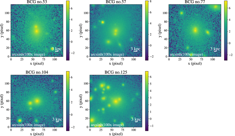
Figure 3. Five additional major mergers identified by visual inspection. These images are displayed in the stretching of arcsinh(100×), and zoomed in to the central 120 pixels (see caption of Figure 1 for more details). The white horizontal bar indicates a scale of 3 kpc.
Download figure:
Standard image High-resolution imageTable 3. The 15 Cores Detected in the Main Sample with Flux Ratio 
| Number | sys_v | v_off_mean | v_off_median | core_ra_im | core_dec_im | flux_ratio | vis |
|---|---|---|---|---|---|---|---|
| 6 | DAP | 365.36 | 389.71 | 131.30121 | 29.308043 | 0.182 | 1 |
| 26 | DAP | −276.83 | −286.22 | 121.4511 | 25.255268 | 0.060 | 0 |
| 40 | DAP | 99.74 | 95.60 | 244.68321 | 25.946503 | 0.110 | 1 |
| 53 | DAP | −125.05 | −110.32 | 125.38854 | 55.153046 | 0.045 | 1 |
| 57 | DAP | 339.90 | 340.83 | 117.48328 | 29.417328 | 0.053 | 0 |
| 57 | DAP | 149.73 | 64.86 | 117.48128 | 29.419292 | 0.011 | 1 |
| 68 | DAP | 75.07 | 70.78 | 205.67506 | 26.23668 | 0.063 | 0 |
| 68 | DAP | 204.02 | 229.98 | 205.67241 | 26.239765 | 0.054 | 0 |
| 72 | DAP | 335.53 | 267.27 | 246.17114 | 25.329369 | 0.115 | 1 |
| 77 | DAP | 50.21 | 47.83 | 219.43756 | 48.590576 | 0.005 | 1 |
| 103 | corrected | −138.94 | −92.70 | 245.36404 | 42.76216 | 0.075 | 0 |
| 103 | corrected | −212.12 | −191.30 | 245.36154 | 42.76228 | 0.395 | 1 |
| 104 | DAP | 257.89 | 237.99 | 244.15991 | 42.448227 | 0.051 | 1 |
| 123 | DAP | 477.52 | 453.52 | 321.44464 | 0.9318187 | 0.147 | 1 |
| 125 | DAP | 185.18 | 141.89 | 127.02314 | 44.76726 | 0.0199 | 1 |
Note. The columns are the BCG ID, source of the systemic velocity, mean and velocity velocity offsets in the core region (in units of km s−1), R.A. & decl. (both in degrees), flux ratio, selection method (vis = 1 denotes cores identified through visual inspection).
Download table as: ASCIITypeset image
3.6. Completeness Correction and the Multiple-core Frequency
The multiple-core frequency in Equation (1) is defined for a volume-limited sample. So far we have been presenting the multiple-core measurements among the 79 BCGs of our Main sample, which does not constitute a volume-limited sample (see below). It is also not yet clear whether our BCG sample, constructed somewhat heterogeneously from the MaNGA primary, secondary, color-enhanced, and two ancillary programs, are a representative subsample of all BCGs at z ≤ 0.15. In this section, we describe our way of applying a completeness correction factor to the multiple-core frequency (also see a more detailed discussion in Section 5.1).
As the SDSS main galaxy sample (Strauss et al. 2002) is r-band limited, van den Bosch et al. (2008) derive a corresponding completeness limit in stellar mass as a function of redshift, after considering the uncertainties in K corrections in converting flux to luminosity, as well as the spread in mass-to-light ratios of red galaxies, appropriate for our BCGs:
where DL is the luminosity distance. We show the distribution of our BCGs in the stellar mass versus the redshift plane (as the large green and red symbols), along with those in the All sample (as orange points) in Figure 4 (top panel). We note that 6 of the BCGs in the Main sample fall short of the completeness limit, and we shall refer to the rest, 73 BCGs, as the "volume-limited" sample (Table 1). The green and red symbols represent stellar mass derived based on the SDSS Petrosian (Petrosian 1976) and model magnitudes. It is clear that the difference is small whether the model or Petrosian magnitudes are used for the BCG selection (note that the former is used in the Y07 catalog).
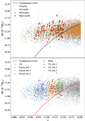
Figure 4. Top: Distribution of stellar mass based on both the model and petrosian magnitudes of our Main sample (large red and green symbols) and All sample (orange and blue dots). The black curve is Equation (3). Bottom: The gray crosses show the distribution of BCGs in our "All" sample (Table 1). They are further split into 3 redshift bins that have about the same comoving volume; for the BCGs above the completeness limit (red line), they belong to our Parent sample (color coded for ease of distinction of the 3 redshift bins). Our volume-limited sample consists of the large circles.
Download figure:
Standard image High-resolution imageTo proceed, we consider all BCGs at z = 0.02–0.15 above the completeness limit and hosted by clusters with M180m
≥ 1014
h−1
M⊙ as the "parent" BCG sample (Table 1). We split the Parent sample into three redshift bins, z = 0.02–0.1025, z = 0.1025 – 0.13, and z = 0.13 – 0.149, which are chosen to have about the same comoving volume. There are 590, 409, 360 BCGs in each bin, among them 22, 26, 25 belonging to our Main sample (Figure 4, bottom panel). For the cores with  , there are 3, 2, 3 in each bin; the numbers for the case with
  are 6, 2, 5, respectively (Table 4). We take the ratio between the number of BCGs in the volume-limited and the Parent sample in each of the redshift bins as a redshift-dependent completeness correction factor. In this way, we obtain a multiple-core frequency of 0.114
29
for the BCGs in the local universe (with
are 6, 2, 5, respectively (Table 4). We take the ratio between the number of BCGs in the volume-limited and the Parent sample in each of the redshift bins as a redshift-dependent completeness correction factor. In this way, we obtain a multiple-core frequency of 0.114
29
for the BCGs in the local universe (with  please note that in this case, whether we use NBCG, mc or
  in Equation (2) gives the same result), which is very close to the value if we simply use the results from our volume-limited sample [fmc = (3 + 2 + 3)/73 =0.0110].
To summarize, including major mergers, there are 10 and 15 confirmed merging systems with flux ratios larger than 0.1 and 0.05, respectively (Figure 2; Table 3). The corresponding "apparent" (i.e., not corrected for completeness) multiple-core frequencies are 0.13 ± 0.04, 0.19 ± 0.05, assuming the error is Poissonian. The volume-limited multiple-core frequency for  is 0.11 ± 0.04. The corresponding value for
  is 0.19 ± 0.05.
The halo mass distributions of the cored BCGs in the Main and volume-limited samples are shown in Figure 5. There are more BCGs with cores in the low halo mass end, but there are also more clusters (hence BCGs) in the low-mass end. We measure the multiple-core frequency in two cluster mass bins  and 14.55–15.1] and find values of fmc = 0.13 ± 0.05 and 0.11 ± 0.08, respectively. Given our sample size, unfortunately we cannot meaningfully measure any cluster mass dependence.
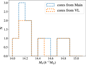
Figure 5. Cluster mass distribution of BCGs with  in the Main (volume-limited) sample, as shown by the blue (orange) histogram. Note that with this flux ratio cut, all the BCGs host only one additional core.
Download figure:
Standard image High-resolution imageHowever, if a higher fmc is indeed found for lower-mass clusters, it could be due to the fact that, as the most massive BCGs tend to inhabit the most massive clusters, and very massive clusters must have started growing a long time ago, the growth of the most massive BCGs happened mostly in the distant past and traces of multiple cores may have now disappeared. At least some of the less massive BCGs (living mostly in less massive clusters) could have grown more recently or be growing now, and therefore would be more likely to show multiple cores.
4. Multiple-core Frequency of Brightest Cluster Galaxies in TNG300
Next we will measure the multiple-core frequency of BCGs from TNG300. As mentioned in Section 2.2, there are 225 BCGs in snapshot 91, which is the output closest to the median redshift of our MPL-9 sample. With the pipeline that can automatically detect cores in imaging data in hand (Section 3.3), in principle it is straightforward to apply it to mock images of simulated BCGs. However, we first need to construct the cluster selection function of our volume-limited sample (Table 1) and apply it to the TNG halos, such that the resulting multiple-core frequency can be better compared with the observed value.
4.1. The Halo Sample
To construct the selection function of the observed BCGs, we consider a subset of the Y07 cluster sample, selected to lie at z = 0.07–0.11 within a randomly chosen area bounded by the R.A. range of 14027–229
90, and decl. range of 5
06–54
89, which corresponds to a comoving volume equal to a TNG300 box. There are, incidentally, also 225 BCGs with cluster mass M180m
≥ 1014
h−1
M⊙, and stellar mass above the completeness limit; we shall refer to this sample as the "TNG-Comparison" sample. Figure 6 shows the distribution of BCGs in the stellar mass versus redshift space of the TNG-Comparison sample (blue points), together with all the BCGs living in massive clusters from the Y07 catalog (i.e., the "All" sample). The cluster mass distributions of the TNG-Comparison sample and the Main sample are shown in Figure 7. The selection function is calculated by computing the ratio of these two distributions as a function of cluster mass. If there are more BCGs in our Main sample than in the TNG-Comparison sample in a mass bin, the value of the selection function is set to 1 in that bin.
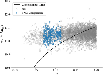
Figure 6. There are 225 BCGs with stellar mass above the completeness limit at z = 0.07 – 0.11 within a (300 Mpc)3 volume from the catalog of Y07, which are referred to as the TNG-Comparison sample (blue points). The corresponding cluster sample is used to construct the halo mass selection function.
Download figure:
Standard image High-resolution image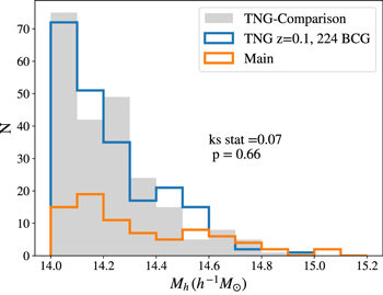
Figure 7. Halo mass distribution in 0.1 dex bins, of the BCGs in the TNG-Comparison (blue histogram), the Main samples (green histogram), and in cluster-scale TNG300 halos (with mass M200m
≥ 1014
h−1
M⊙, orange histogram). The halo mass selection function is constructed by the ratio of the first two distributions. The median masses of the two observational samples are  and 14.25, respectively. Performing a two-sample Kolmogorov–Smirnov test between the TNG300 and TNG-Comparison samples, we obtain a p-value of 0.66, supporting the assumption that they are drawn from the same parent population.
Download figure:
Standard image High-resolution imageAs the second step, we examine whether the halo mass distributions of the TNG300 halos and that of the TNG-Comparison sample are similar. Before doing so, we have to remove a simulated BCG. 30 By comparing the 224 halos from TNG300 with 225 clusters from the TNG-Comparison, we show in Figure 7 that the mass distributions of the two are similar. Performing a two-sample Kolmogorov–Smirnov (K-S) test, we obtain a K-S statistic of D = 0.07, and p-value of 0.66, supporting the assumption that they are drawn from the same parent population.
We now can then safely apply the selection function to the TNG sample, which is done in a Monte Carlo fashion. For each TNG BCG, we draw a random number between 0 and 1 and compare it with the value of the selection function corresponding to the halo mass of that BCG. If it is smaller, we accept the BCG/halo. Repeating this for all 224 TNG BCGs, we then have one "mock" BCG/halo sample, whose halo mass distribution should be similar to our volume-limited sample. For statistical robustness, we have constructed 50 such mock samples. One of the mock BCG/halo samples is shown in Figure 8. We then measure the multiple-core frequency from these 50 samples in the following sections.
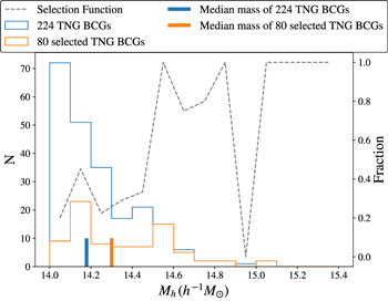
Figure 8. Halo mass distribution of one of the 50 mock TNG samples. In this example, 80 of the 224 TNG BCGs are selected, with halo mass distribution consistent with that in our TNG-Comparison sample. The gray dashed line is the selection function.
Download figure:
Standard image High-resolution image4.2. Synthetic Images
The synthetic images are generated following the procedures described in Rodriguez-Gomez et al. (2019). The observing angle is perpendicular to the xy plane. The pixel size is 0.396'' as in the SDSS, and the field of views are 1000 × 1000 pixels and 800 × 800 pixels, matching those of the real BCGs. As BCGs mainly consist of old stellar populations with little dust (von der Linden et al. 2007), the images are generated by the stellar population synthesis code GALAXEV (Bruzual & Charlot 2003), and we have skipped the radiative transfer calculations (for justification, please see Rodriguez-Gomez et al. 2019). After the idealized i-band images are generated (in units of nanomaggies, as in SDSS images), they are convolved with a Gaussian point-spread function (PSF) with 1.5'' FWHM. Adding the model images to a patch of real SDSS sky centered at (R.A., decl.) = (193°, 33°) that is void of bright galaxies and stars completes the generation of synthetic images. We show an example image in Figure 9.
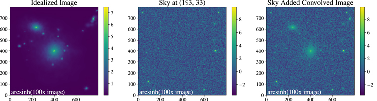
Figure 9. The left panel is the idealized image of a BCG in TNG300 generated by the method described in Rodriguez-Gomez et al. (2019). The middle panel is an SDSS image centering at (R.A., decl.) = (193, 33) degree. The right panel is the product of convolving the left panel with a Gaussian PSF then adding the sky in the middle panel. As noted in Figure 1, the values shown on the color bars correspond to arcsinh(100× flux/nanomaggy).
Download figure:
Standard image High-resolution image4.3. Photometry
The photometry of TNG BCGs is obtained in a similar fashion as described in Section 3.1. We feed the 1000 × 1000 pixel synthetic images to SExtractor, with BACK_SIZE = 200 (1/5 of the image size), to obtain their segmentation maps. We subtract the SExtractor measured background from the images, mask out the region of the sources touching the BCGs, and substitute the region of other sources with a Gaussian noise that has the standard deviation of the sky. These "BCG-only" images are fed to Ellipse to obtain empirical surface brightness models and profiles. We then subtract the empirical models from the synthetic images to obtain residual maps. Also, we fit a single Sérsic profile to the surface brightness profile in order to obtain the total flux and Re of the BCGs.
Two BCGs have complex profiles that cannot be fit by a single Sérsic profile. We use the part of their curve of growth from Ellipse within 150 kpc and above the sky uncertainty to obtain their total flux and Re (please see Appendix A for more details). We also visually inspect all of the profiles and residuals, and find that six BCGs have unreliable profiles that are affected by bright neighbors in the field (please see Appendix B.4.3). As this fraction is small and should be independent of the multiple-core frequency, we add a warning flags to them and remove them from the further analyses. However, one of them (ID 65561) actually has a double-core structure, and we shall report the multiple-core frequency with and without these six BCGs in Section 4.6. In total 218 simulated BCGs have good photometry measurements.
4.4. Identifying Multiple Cores
The identification of cores for the TNG BCGs is performed in the same fashion as described in Section 3.3. The only difference is the criteria of maximum separation due to the Re
difference between the Main sample and the simulated sample. We compare the Re
distribution of each of the 50 mock TNG samples with the Main sample using the K-S test, and find some differences, which could be due to the IFU coverage criterion imposed on the observed samples (see also Section 5.1.1 and Figure 15). The average value of median Re
for the 50 mock samples is 22.35 h−1 kpc, and the median Re
of the Main sample is 16.10 h−1 kpc. We thus modify the 18 kpc separation adopted in Section 3.2 by the ratio of  and set 25 kpc as the maximum separation for the search of cores in simulated BCGs. To mimic what is done to the real BCGs, a minimum search radius of 2.5 kpc is also set.
We run SEP with the strong deblending parameters 31 and a low detection threshold to detect any possible core within 2.5–25 kpc from the BCG center on the residual maps.
4.5. Flux Ratio
The procedures are similar to that described in Section 3.5. For the flux of the cores, we consider the maximum value among six types of measurements, including: (i) the sum of pixels in the SEP segmentation region extracted from the images, and (ii)–(vi) the sum of the pixels within a radius of 1, 2... to 5 kpc of the cores. Fourteen cores are found to have  . There are 7 additional major mergers selected by visual inspection (Figure 10). Therefore, 21 cores have
  . We note that the one BCG that is excluded due to bad photometric fit (Section 4.1) actually has two cores.
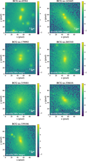
Figure 10. Zoom-in images of the extra seven major mergers in TNG selected by visual inspection. The white horizontal bar indicates a scale of 3 kpc.
Download figure:
Standard image High-resolution imageAs the synthetic images only use stellar particles that belong to the FoF group to which a simulated BCG belongs to, there is no "contamination" from foreground/background objects. Therefore, unlike in the case for MaNGA BCGs, we do not further confirm the physical association of cores with the BCGs via kinematics.
4.6. Results
The multiple-core frequency of BCGs having  among the full TNG sample is 21 out of 218, or fmc = 0.10 ± 0.02. It is 23 out of 225 (fmc = 0.10 ± 0.02) if including BCGs without good photometry (Table 5). For the case of
  , the numbers are 37 out of 218 (fmc = 0.170) or 39 out of 225 (fmc = 0.173). Note that these are values obtained without applying the observed halo selection function and thus should not be directly compared with our observational results.
Table 4 . Statistics of Core Detection
| Redshift Range | 0.02–0.1025 | 0.1025–0.13 | 0.13–0.149 |
|---|---|---|---|
| Parent sample | 590 | 409 | 360 |
| Volume-limited (VL) sample | 22 | 26 | 25 |
Core number with  in VL in VL | 3 (6) | 2 (2) | 3 (5) |
| Core number expected in Parent | 80.5 | 31.5 | 43.2 |
Multiple-core frequency ( ) ) | 0.140 | 0.077 | 0.120 |
Multiple-core frequency ( ) ) | 0.273 | 0.077 | 0.200 |
Download table as: ASCIITypeset image
Table 5. The Cores of the 225 BCGs in TNG300
| ID | core_Δx | core_Δy | flux_ratio | visual |

|
|---|---|---|---|---|---|
| 22739 | 11.5535 | −6.9935 | 0.202 | 1 | 14.832 |
| 65561 | 1.9560 | 1.9410 | 0.002 | 1 | 14.594 |
| 65561 | 3.4750 | 15.0028 | 0.172 | 1 | 14.594 |
| 143445 | 6.8048 | −9.0130 | 0.050 | 1 | 14.288 |
| 154823 | 17.4887 | −5.7579 | 0.101 | 0 | 14.351 |
| 179992 | 0.6054 | 6.5247 | 0.093 | 1 | 14.307 |
| 197011 | 16.3293 | 9.3378 | 0.106 | 0 | 14.262 |
| 200512 | 7.6236 | 1.3997 | 0.117 | 1 | 14.260 |
| 216339 | 8.3862 | −11.3124 | 0.220 | 1 | 14.217 |
| 228396 | 14.1833 | −0.7329 | 0.149 | 0 | 14.211 |
| 237651 | −8.9273 | 4.0888 | 0.194 | 1 | 14.053 |
| 265310 | −1.1209 | −4.5295 | 0.002 | 1 | 14.154 |
| 267972 | −11.2348 | 2.3378 | 0.183 | 0 | 14.112 |
| 267972 | −15.1513 | 4.1710 | 0.126 | 0 | 14.112 |
| 269979 | 8.1404 | −14.0914 | 0.116 | 1 | 14.125 |
| 292034 | −3.1866 | −16.8615 | 0.134 | 0 | 14.091 |
| 296390 | −7.1637 | 10.8193 | 0.115 | 0 | 14.046 |
| 308262 | −14.6869 | 12.4339 | 0.116 | 0 | 14.029 |
| 308262 | −13.2060 | 14.6144 | 0.114 | 0 | 14.029 |
| 311982 | 10.5523 | 3.9004 | 0.112 | 0 | 14.047 |
| 319481 | −2.0510 | −5.1047 | 0.003 | 1 | 14.010 |
| 336616 | −3.5629 | 3.3941 | 0.010 | 1 | 14.007 |
| 339186 | −0.8054 | 5.3912 | 0.003 | 1 | 14.018 |
Note. The columns are the subhalo ID, their position with respect to the BCG in h−1 ckpc, the flux ratio, and the visual inspection flag (where 1 denotes identification via visual inspection; see Figure 10), host halo mass (in h−1 M⊙). No. 65561 is an excluded BCG with bad photometry (with two cores).
Download table as: ASCIITypeset image
The multiple-core frequencies of the 50 mock samples for the case of  are shown in Figure 11; the median value is 0.076, with a standard deviation of 0.027. The multiple-core frequency is thus formally fmc = 0.08 ±0.02 (Poisson) ± 0.03 (Systematic). Hereafter we shall combine the two uncertainty terms and quote fmc = 0.08 ± 0.04. For the case of
  , we find that fmc = 0.14 ±0.03 (Poisson) ± 0.03 (Systematic). We also test the Monte Carlo method by running 100 and 200 ensembles, finding that they have nearly the same median and standard deviation as those of 50 ensembles.
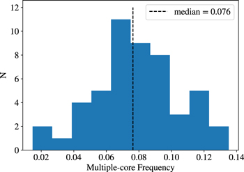
Figure 11. Distribution of the multiple-core frequency of the 50 mock TNG samples, for the case of  . The median is 0.076, and the standard deviation is 0.027.
Download figure:
Standard image High-resolution imageThe halo mass distribution of BCGs with multiple cores is shown in Figure 12. It is clear that most of the cores are detected in BCGs with lower halo mass, which explains why the multiple-core frequency becomes lower after the selection function is applied, as the selection function filters out more halos at the low-mass end.
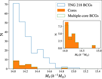
Figure 12. Halo mass distribution of simulated BCGs with  (green histogram), compared to that of the full TNG sample with good photometry (218 BCGs; blue histogram). As a BCG can host more than one core, we also show the distribution of cores as the orange histogram, where each core contributes to the counts. The inset shows more clearly the numbers of cores and BCGs.
Download figure:
Standard image High-resolution imageThe multiple-core frequency of our Main sample (the black dot in Figure 13) is slightly higher than that of the TNG sample (the purple dot in Figure 13), although the discrepancy is only at 1σ level.
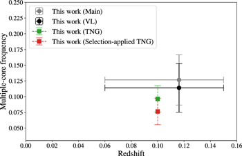
Figure 13. Comparison of our observed and simulated multiple-core frequencies fmc. The gray and black points are from the Main and volume-limited samples, respectively. The error bars in redshift represent the redshift range of the samples. The error bars of the multiple-core frequencies are Poissonian. The green point (fmc = 0.0963) is the result based on the whole TNG sample, while the red point (fmc = 0.0763) is the average over the 50 mock samples. Note that these values follow the definition of fmc and thus a BCG would be counted N times if it has N cores. If we only consider unique BCGs, the values of the green and red points will be reduced by 11% and 7%, respectively.
Download figure:
Standard image High-resolution imageAs in Section 3.6, we also measure the multiple-core frequency in two halo mass bins ( and 14.55–15.1). The values are 0.1 ± 0.2 and 0.06 ± 0.06, respectively. Again the limited halo sample size prevents us from measuring any halo mass dependence.
5. Discussion
After having measured the multiple-core frequency from both MaNGA (Section 3) and IllustrisTNG (Section 4), here we discuss the robustness of our sample selection (Section 5.1), showing it is representative of the local BCGs. We compare our results with findings from the literature in Section 5.2, measure the mass growth rate of BCGs in IllustrisTNG (Section 5.3) and finally discuss the effect of the presence of cores in the supermassive black hole radio activity (Section 5.4).
5.1. Velocity Offsets of the Cores and Sample Selection
Velocity offset distribution shown in Figure 2 is slightly skewed to the positive side and is independent of the redshift of the BCGs. It is not clear what causes the skew. We have visually inspected the DAP velocity maps of the cored BCGs, and confirmed that indeed more cores show higher velocity than the main body of the BCGs and that the spectral fits to the cores are adequate.
One may question how representative our BCG sample (e.g., the Main or volume-limited samples) is, with respect to the overall BCG population. This is a legitimate concern, as (1) the MaNGA sample is constructed to have a flat stellar mass distribution, thus very massive galaxies, like BCGs, could be overrepresented, compared to a volume-limited sample; (2) our BCGs are assembled from MaNGA's primary, secondary, and color-enhanced samples, as well as the BCG and MASSIVE ancillary programs, which makes the selection a bit heterogeneous. We show in the following that our sample selection criteria do not result in a biased sample of BCGs.
5.1.1. Unbiased Sample Selection
In Figure 4 (top panel) we see that the stellar mass distributions of BCGs in our Main sample is similar to that of the All sample (Table 1). For a more quantitative analysis, we compare various properties of our volume-limited sample with a subset of clusters from Y07, which is obtained by excluding the MPL-9 BCG sample from the Parent sample, and will be referred to as the "not-in-MaNGA (NIM)" sample (Figure 14; Table 1). Similarly to what we have done in Section 3.6, we make the comparison in three redshift bins of comparable comoving volume (z = 0.02–0.1025, 0.1025–0.13, 0.13–0.149; hereafter bins 1, 2, and 3). There are 529, 376, 332 (22, 26, 25) BCGs in each bin of the NIM (volume-limited) sample. The properties we compare are halo mass, Petrosian half-light radius, Petrosian color, and the number of neighbors, where the neighbors are defined by a certain range in projected distance and redshift (Figure 15). These properties are obtained either directly from the Y07 catalog, or derived from the galaxy member catalog associated with the primary Y07 catalog. We compare these properties through their mean values and the K-S test.
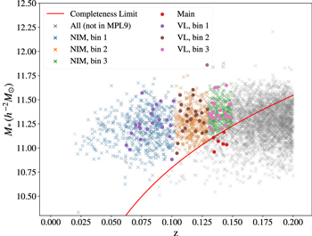
Figure 14. Illustration of the samples used in Section 5.1.1: the blue, brown, and green crosses are our "not-in-MaNGA (NIM)" sample (split into three redshift bins that have about the same volume), which is constructed by excluding the MPL-9 sample from the Parent sample. The completeness limit is represented by the red line. Our volume-limited sample, also split into the same three redshift bins, is shown as large circles.
Download figure:
Standard image High-resolution image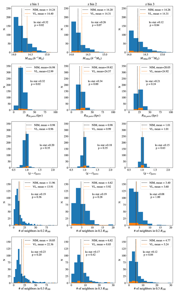
Figure 15. Comparisons of various properties between our volume-limited sample (orange histograms) and the not-in-MaNGA (NIM) sample (blue histograms). From left to right, we show the results from the three redshift bins (z = 0.02 − 0.1025, 0.1025 − 0.13, 0.13 − 0.149); from top to bottom, the properties being considered are cluster mass, half-light radius, g − r color, number of neighbors within 0.2R180m , and the number of neighbors within 0.3R180m , respectively. Based on K-S tests, we see that only the R50 distributions in bins 1 and 2 and the halo mass distribution in bin 1 are different.
Download figure:
Standard image High-resolution imageIn Figure 15, the three columns represent results in each redshift bin, while the rows, from top to bottom, show comparisons in cluster mass, Petrosian half-light radius R50, g − r color, number of neighbors within 0.2R180m , and the number of neighbors within 0.3R180m , respectively. We only consider the Petrosian color within the range of 0.5–2.1, to avoid unreasonable photometry. In all panels, the blue (orange) histograms are for the NIM (volume-limited) sample. Through the two-sample K-S test, we see that only the R50 distributions in bins 1 and 2 and the halo mass distribution in bin 1 are different. For all other properties in all bins, we do not see obvious deviation for our volume-limited sample from the NIM sample. The differences in bin 1 are likely due to the IFU coverage criterion we impose, which translates to a lower redshift limit at z ≈ 0.06 for the observed samples. If we change the lower redshift limit of bin 1 for the NIM sample to 0.06, there is then no significance difference in the halo mass distribution.
In the next section we shall look more into bin 2 to examine the multiple-core frequency obtained from our IFU-based observations and that inferred from imaging data only.
5.1.2. An Independent Estimate of the Multiple-core Frequency
As a further test, we run the core detection procedure as described in Section 3.3 on the SDSS images of the 376 BCGs in bin 2. We choose bin 2 because (1) its redshift is closest to that of our Main sample, and (2) there seems to be some difference in R50 between our volume-limited sample and the NIM sample (Figure 15). Among these, two BCGs do not have a good Ellipse model. The core detection pipeline finds 186 cores in the remaining 374 BCGs. We fit Sésic profiles to the Ellipse curve of growth to obtain their total flux. 18 cores have  . We also visually select additional 14 major mergers. The multiple-core frequency is thus fmc =0.09 ± 0.02, which is shown in the right panel of Figure 16 as the brown point.
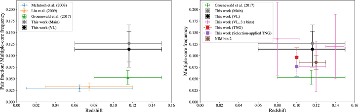
Figure 16. Left: Comparison of our multiple-core frequency with pair fraction from the literature. The error bars in redshift represent the redshift range of the samples. The measurements from the literature are plotted at the middle point of their redshift ranges, and the result of this work is plotted at the mean redshift of our samples. Right: Similar to Figure 13, but showing also the result from redshift bin 2 of the not-in-MaNGA (NIM) sample (brown point), as well as the pair fraction from Groenewald et al. (2017, G17; green point). The pink points represent the values derived from our volume-limited sample, split in three redshift bins.
Download figure:
Standard image High-resolution imageGiven that there is minimum selection involved in this sample, ideally the multiple-core frequency based on this subsample should be consistent with that of the full TNG sample (i.e., without the selection function applied). They indeed are consistent (see the brown and red points). It is also interesting to note that these values are also close to what we obtain from the volume-limited sample, when similarly split into three redshift bins (i.e., the pink point at z ≈ 0.12). One should bear in mind that no spectroscopic confirmation is performed for the cores detected in the NIM sample, and thus the value quoted above should be regarded as an upper limit. However, given our conclusion that most of the imaging-detected cores are actually physically associated with the BCGs as confirmed by kinematics (28 out of 30; see Section 3.4), the difference from the true value may be small.
5.2. Comparison with the Literature
Figure 16 (left panel) shows a comparison of our measurements with some of the previous works that measure merger rates of BCGs at redshift ranges similar to ours (McIntosh et al. 2008; Liu et al. 2009; Groenewald et al. 2017; hereafter M08, L09, and G17, respectively). It should be noted that the BCG selection and the the merger definition are different among these works.
All of M08, L09, and G17 focus on major mergers within 30 kpc. The sample of M08 is volume-limited and has halo mass ≥ 2.5 × 10¹³ M⊙; the G17 sample is also volume-limited, but has a much higher halo mass threshold of ≥ 2.9 × 10¹⁴ M⊙. The sample of L09 does not provide an estimate of the halo mass. M08 and G17 select pairs with mass ratios larger than 0.25, while the sample of L09 has an average luminosity ratio of 0.5. Moreover, M08 and L09 select physically related pairs by the distorted morphology. G17 select close pairs and apply a correction factor derive from a smaller spectroscopic confirmed subsample (12 pairs). They apply a limit in velocity difference of 300 km s−1, and conclude that a limit on 500 km s−1 only increases the fraction by about 0.03%.
Given the difference between our approach and that of others, it is not easy to directly compare our multiple-core frequency with the major merger pair fractions in previous works. There are differences in sample selection, maximum separation and, most importantly, the method of finding physically related pairs. G17 note that the morphology distortion is more obvious in the late stage of the mergers (Lotz et al. 2011); hence it is possible to obtain a lower pair fraction if relying on the distortion in galactic shape only.
Brough et al. (2011) conduct the first targeted IFS observation of BCGs with close companions, with the goal of determining the merger rates, using the Visible Multi-Object Spectrograph on the Very Large Telescope. They select three BCGs with companions and one without companions within 10'' (18 kpc at z ∼ 0.1). These BCGs are from the sample of the 625 BCGs from von der Linden et al. (2007) selected from the C4 catalog (Miller et al. 2005). 20% of these BCGs have visually identified massive companions. They find that two out of three companions are likely bound with their BCGs. Jimmy et al. (2013) apply the same method to 10 BCGs, of which seven with companions and the rest without. They use the "G-M20" merger selection criteria (Lotz et al. 2008) and conclude that 4 out of 10 BCGs have gone through mergers within the past 0.2 Gyr, although their sample selection might be biased toward BCGs that have companions.
5.3. Mass Growth Rate of BCGs
The mass growth rate of massive galaxies (for which BCGs stand at the extremal end) has been an important topic in galaxy formation. Traditionally this is usually done through comparisons of luminosity or stellar mass functions (SMF) measured at different cosmic epochs (e.g., Scarlata et al. 2007; Bernardi et al. 2013; Bundy et al. 2017). For example, Bundy et al. (2017) have used a large sample of massive galaxies extracted from the SDSS stripe 82 and concluded that there is very little evolution of the massive end since z ∼ 0.7. They suggest that any galaxy growth would have occurred at the outskirts beyond the observational aperture, which corroborates one critical aspect of all SMF measurements at the massive end, namely proper measurements of the "total" luminosity of the galaxies, a challenge that we also face in this study. For example, using a careful sky subtraction and sophisticated modeling technique, Bernardi et al. (2013) show that the abundance of massive galaxies could have been underestimated by a dex in previous studies (see also Huang et al. 2018). Another approach is to use the Hubble diagram of BCGs (Aragon-Salamanca et al. 1998; Whiley et al. 2008).
A different approach is employed by Masjedi et al. (2008), who use the cross-correlation function between the spectroscopic sample of luminous red galaxies (LRGs) and photometric galaxies to infer the very small scale clustering of LRGs, from which they are able to infer a growth rate of ∼2% per Gyr measured at z ≈ 0.25.
Given the consistency in multiple-core frequency between our volume-limited sample and the TNG300, in principle we can infer the mass growth rate of BCGs, using directly the information derived from the simulation. For each of the 225 BCGs in TNG300, we trace the stellar mass content within a 25 kpc radius out to z = 0.6, and compute the average growth rate, which is the mass difference between z = 0.6 and 0.1 divided by the time lapse between these two epochs (4.5 Gyr). The median (mean) of the mass growth rate is found to be 1.3%/Gyr (4.1%/Gyr).
5.4. Nuclear Radio Activity
By matching our Main sample to the radio galaxy catalog presented in Lin et al. (2018),
32
we find that 35% of the BCGs have 1.4 GHz radio power P1.4 > 1023 W Hz−1 (a threshold typically used to separate star formation-powered and nuclear-powered radio activity), which is similar to the results shown in (Lin & Mohr 2007, Table 5 therein). For the 30 BCGs with cores (irrespective of their  values), the fraction is similar (33%). However, if we focus on 10 BCGs with
  , the fraction increases to 50%. It is tempting to attribute to the elevated radio activity to the mergers with massive satellites, but given the small number of the BCGs, we do not attempt to further interpret the finding. We note, however, if we increase the radio power threshold (e.g., to P1.4 > 1024 W Hz−1), the presence of cores only makes a small enhancement in the radio-loud fraction compared to the BCGs without multiple cores (20% v.s. 18%).
6. Conclusion and Prospects
The motivation of this work is to solve the discrepancy of stellar mass growth of BCGs at z < 0.5 between models and observations, which may be caused by the use of fixed aperture photometry adopted in observations. To tackle this problem, deep photometry of BCGs and careful work on sky subtraction are required.
On the other hand, studying the merger rate in the inner regions of BCGs can be a good alternative to solving this discrepancy. However, studying merger rates requires the combination of the frequency of multiple cores and merger timescale, and the latter needs to come from simulations. Hence, in this work we focus on the multiple-core frequency, which is a direct observable.
We have used the largest sample of BCGs with IFS data—about 7 times larger than previous attempts—to study the BCG multiple-core frequency, defined to be the fraction of BCGs that host one or more physically associated dense cores (with core-to-total flux ratio ≥0.1 and velocity offset ≤500 km s−1) in a volume-limited sample. Our observational result, fmc = 0.11 ± 0.04, appears to be consistent with the state-of-the-art cosmological hydrodynamical simulation IllustrisTNG (fmc = 0.08 ± 0.04), which is small compared to the discrepancy in the stellar mass growth revealed in some of the earlier works. Our results are not very sensitive to sample selection, as long as it is volume limited.
Thus, we may have obtained a better understanding of the stellar mass assembly of BCGs: while the discrepancy in the growth of "total" mass may be due to the different apertures used in observations and simulations (e.g., Ragone-Figueroa et al. 2018), the multiple-core frequency in the innermost part of the BCGs appears to be comparable in observations and theory. Given such a reasonable agreement, we further trace the formation history of simulated BCGs back to z = 0.6 and obtain a mean growth rate of 4.1% per Gyr within the central 25 kpc radius.
Our main conclusions are:
- 1.Cores detected based on images often are indeed associated with their BCGs (about 93% of the time), although stars need to be carefully removed.
- 2.It is important to have realistic simulated images for the observation versus simulation comparisons. Applying stellar population synthesis modeling, effects of PSF, and sky noise are all critical.
- 3.Cores are mostly detected in BCGs of low-mass clusters (around 1014 h−1 M⊙), which may be mainly because of the higher abundance of such clusters (although it might also be due to different evolutionary stages of low-mass clusters compared to more massive ones; please see the discussion at the end of Section 3.6).
- 4.We obtain a multiple-core fraction of 0.11 ± 0.04 at z ≈ 0.1 within a 18 kpc radius from the center, which is comparable to the value of 0.08 ± 0.04 derived from mock observations of 218 simulated BCGs in IllustrisTNG300 at z = 0.1.
We have established that cores seen in BCGs are most likely to be physically associated, and therefore one can obtain a rough estimate of multiple-core frequency purely based on imaging data (e.g., Section 5.1.2). However, in principle, the IFS data could further allow a detailed investigation of the properties of the cores, such as the stellar populations of the satellites that are in the process of merging with the BCG. We shall leave such an analysis applying to the full MaNGA BCG sample to a future study. In addition, we are not able to determine whether there is a dependence on halo mass of fmc, both in observations and simulations. For the latter, this could be somewhat mitigated by taking three projection directions per simulated halo (currently we only consider the projection along the simulation z-axis), and also considering more snapshots between z = 0.06 and 0.15, and by considering lower-mass halos (e.g., down to the group regime), so that the simulation statistics could be greatly boosted, potentially enough to search for such trends.
The fully automatic pipeline we developed can be readily applied to the whole MaNGA sample (MPL-11; already fully public). However, it is still critical to conduct visual inspection of BCGs, as these systems often are too challenging even for the most sophisticated software. Nevertheless, the pipeline can be readily applied to deep images from Hyper Suprime-Cam (Aihara et al. 2018) or data from the upcoming Rubin Observatory's Legacy Survey of Space and Time, 33 and slitless spectroscopy from Roman Space Telescope 34 or Euclid 35 to study the multiple-core frequency at higher redshifts, where mergers are expected to take place more often.
This kind of study can also be extend to lower-mass clusters and groups (Banks et al. 2021), which may provide more stringent constraints, given the much higher abundance of groups.
We thank Gabriel Torrealba for developing the Ellipse package used in this work. We are grateful to Wei-Hao Wang, Kyle Westfall, James Lottes, Andrew Cooper, David Wake, Michael Blanton, Xiaohu Yang, and Ting-Wen Lan for helpful comments, and Taira Oogi and Abdurro'uf for help with handling of simulated and MaNGA data, respectively. We thank an anonymous referee whose comments have improved the clarity of the paper. Y.H.H. and Y.T.L. are grateful for support from the Ministry of Science and Technology of Taiwan under grants MOST 110-2112-M-001-004 and MOST 109-2112-M-001-005, and a Career Development Award from Academia Sinica (AS-CDA-106-M01). D.N. acknowledges funding from the Deutsche Forschungsgemeinschaft (DFG) through an Emmy Noether Research Group (grant No. NE 2441/1-1). Y.T.L. thanks I.H., L.Y.L. and A.L.L. for constant encouragement and inspiration.
Funding for the Sloan Digital Sky Survey IV has been provided by the Alfred P. Sloan Foundation, the U.S. Department of Energy Office of Science, and the Participating Institutions. SDSS acknowledges support and resources from the Center for High-performance Computing at the University of Utah. The SDSS website is www.sdss.org.
The SDSS is managed by the Astrophysical Research Consortium for the Participating Institutions of the SDSS Collaboration including the Brazilian Participation Group, the Carnegie Institution for Science, Carnegie Mellon University, Center for Astrophysics ∣ Harvard & Smithsonian (CfA), the Chilean Participation Group, the French Participation Group, Instituto de Astrofísica de Canarias, The Johns Hopkins University, Kavli Institute for the Physics and Mathematics of the Universe (IPMU)/University of Tokyo, the Korean Participation Group, Lawrence Berkeley National Laboratory, Leibniz Institut für Astrophysik Potsdam (AIP), Max-Planck-Institut für Astronomie (MPIA Heidelberg), Max-Planck-Institut für Astrophysik (MPA Garching), Max-Planck-Institut für Extraterrestrische Physik (MPE), National Astronomical Observatories of China, New Mexico State University, New York University, University of Notre Dame, Observatório Nacional/MCTI, The Ohio State University, Pennsylvania State University, Shanghai Astronomical Observatory, United Kingdom Participation Group, Universidad Nacional Autónoma de México, University of Arizona, University of Colorado Boulder, University of Oxford, University of Portsmouth, University of Utah, University of Virginia, University of Washington, University of Wisconsin, Vanderbilt University, and Yale University.
The IllustrisTNG simulations were undertaken with compute time awarded by the Gauss Centre for Supercomputing (GCS) under GCS Large-Scale Projects GCS-ILLU and GCS-DWAR on the GCS share of the supercomputer Hazel Hen at the High-performance Computing Center Stuttgart (HLRS), as well as on the machines of the Max Planck Computing and Data Facility (MPCDF) in Garching, Germany.
This work has made use of data from the European Space Agency (ESA) mission Gaia (https://www.cosmos.esa.int/gaia), processed by the Gaia Data Processing and Analysis Consortium (DPAC, https://www.cosmos.esa.int/web/gaia/dpac/consortium). Funding for the DPAC has been provided by national institutions, in particular the institutions participating in the Gaia Multilateral Agreement.
Appendix A: Consistency of Photometry between Ellipse and PyMorph
In this section, we compare all kinds of the photometry we have used and show that they are consistent (to the degree of our needs). In Section 3.1, we have described the two sources of photometry of our BCGs, namely that based on PyMorph and from Ellipse. The former (hereafter PyMorph) is from the photometric catalogs of M16 and F19 (please refer to that section for the procedures of combining the best models in these two catalogs for the photometry of 74 BCGs, which shall be referred to as the UPenn sample). The latter (Ellipse-based) also provides two kinds of measurements: one is the Sérsic fitting mentioned in Section 3.1 (hereafter Sérsic), and the other is the photometry within 150 kpc mentioned in Section 4.3 (hereafter 150 kpc). The priority order in our usage is PyMorph, Sérsic, then 150 kpc. As PyMorph and Sérsic are parametric models that can be integrated to infinity, while the 150 kpc one is an empirical model that sums up the flux within a finite radius, the total flux from 150 kpc should be systematically smaller than the parametric models. To understand the differences among the three photometric measurements and to check whether they are consistent, here we compare the photometry based on the UPenn sample.
Figures 17 and 18 show the profiles of the three kinds of photometry for an example BCG, No. 31, in our Main sample. The profiles, as well as the half-light radii, are functions of the radius of the generalized ellipse profile in units of kiloparsec (Peng et al. 2002). The radius or radial coordinate of the generalized ellipse profile is defined as:
where (xc , yc ) is the center, q is the axis ratio, and C0 is the "boxiness" parameter (C0 = 0 corresponds to a perfect ellipse; in running Ellipse this is the value we adopt).
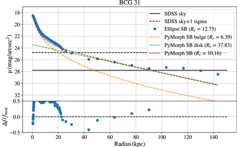
Figure 17. Example (BCG No. 31) of the surface brightness profiles of Ellipse and the two-component model of PyMorph. The upper panel shows the surface brightness profile from Ellipse within 150 kpc (blue dots), the bulge component from PyMorph (orange dashed line), the disk component from PyMorph (green dashed line), and the combination of the two (red dashed line). The surface brightness profiles, as well as the half-light radius, are presented as a function of the radius of the generalized ellipse profile in units of kiloparsec. The sky and sky uncertainty measured by SExtractor are also shown. The lower panel shows the difference between two profiles as (flux Ellipse − flux Pymorph )/flux Pymorph .
Download figure:
Standard image High-resolution image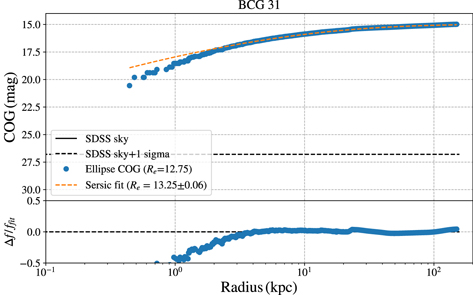
Figure 18. Example (BCG No. 31) showing the curve of growth out to 150 kpc from Ellipse (blue points) and a single Sérsic fitting to the profile (orange curve). The curve of growth, as well as the half-light radius, are presented as functions of the radius of the generalized ellipse profile in units of kiloparsec. The lower panel shows the difference between two profiles as (flux Ellipse − flux Sersic )/flux Sersic .
Download figure:
Standard image High-resolution imageMost of the surface brightness profile of PyMorph and 150 kpc are consistent down to the sky level, but the 150 kpc ones are more sensitive to the light of cores, nearby neighbors, and other asymmetric structures. For example, there are two cores at around 20 kpc of BCG No. 31 that causes a "bump" (see Figure 19).
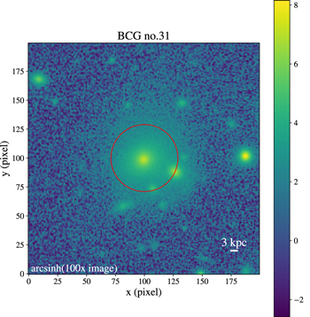
Figure 19. Image of BCG No. 31, zoomed in to the central 200 pixels. The red circle has a radius of 20 kpc and touches two satellites, which cause a dip in the surface brightness profile derived by Ellipse.
Download figure:
Standard image High-resolution imageBelow we provide pairwise comparison of the three kinds of photometric measurements. First, in Figure 20 we show the comparison of the total flux (left panel) and half-light radius (middle panel) of PyMorph and 150 kpc of the UPenn sample. For both quantities, the values based on 150 kpc are slightly smaller. There is also an outlier to the distribution. Upon inspection of the surface brightness profiles, we deem that the values based on 150 kpc are incorrect (presumably due to its sensitivity to the residuals from bright neighbors). The panel on the right shows the comparison based on whole UPenn sample, zoomed in to the range around zero.
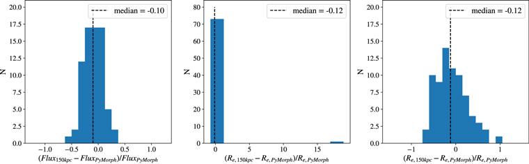
Figure 20. Comparison of total flux (left panel) and Re (middle panel) from 150 kpc and PyMorph of the UPenn sample of 74 BCGs. The panel on the right is a zoom-in to values around zero for Re .
Download figure:
Standard image High-resolution imageSecond, we compare the Sérsic and PyMorph of the UPenn sample in Figure 21 (again, left panel for the total flux, and middle panel for Re ). There are four BCGs that have Δflux > 50%. The panel on the right shows the comparison based on whole UPenn sample, zoomed in to the range around zero.
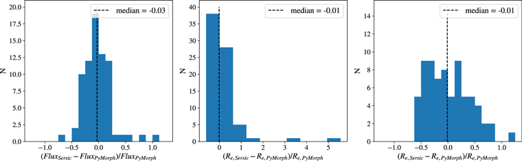
Figure 21. Comparison of total flux (left panel) and Re (middle panel) of Sérsic and PyMorph of the UPenn sample. The panel on the right is a zoom-in to values around zero for Re .
Download figure:
Standard image High-resolution imageThe comparison between 150 kpc and Sérsic is presented in Figure 22, which shows that the total flux of these two method are very consistent and the Re of Sérsic is only larger by 7%.
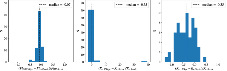
Figure 22. Comparison of total flux (left panel) and Re (middle panel) of 150 kpc and Sérsic of the UPenn sample. The panel on the right is a zoom-in to values around zero for Re .
Download figure:
Standard image High-resolution imageFor the total flux, we use PyMorph and Sérsic for the Main sample, and primarily Sérsic for the simulated sample (except for a few for which 150 kpc is used). The offsets between these distribution are within 7%, although the spread can up to 50%. This is because PyMorph has a better background subtraction and uses a two-component model, so we primarily use it. The flux of 150 kpc is only measured in a limited radius and is systematically smaller than the others, so it is the last choice among the three. The TNG sample does not have the PyMorph measurements, so Sérsic is preferred.
To decide the maximum separation of cores, we use the median Re of PyMorph for the real data, and Sérsic for the mock observations. The PyMorph median Re for the Upenn sample is 17.49 kpc, while that from Sérsic is 17.88 kpc. Based on Figure 21, we expect the two median values to be consistent within 1%. This is because Sérsic and 150 kpc are based on empirical photometry that is more sensitive to the residuals of the bright neighbors. Also, the spread in Re is much larger than the total flux, so a fixed value (18 kpc) is better for direct comparisons between the observation and simulation.
Appendix B: Notable Objects
In the Main sample, several BCGs pose challenges to our pipeline, and we have to apply special treatments for them instead of the general procedure described in Sections 3.3 and 3.4 (see Figure 23). In the simulated sample, for two simulated BCGs we use the Ellipse total flux within 150 kpc instead of results from the single Sérsic fit. We discuss these objects case by case in this Appendix. We also show explicitly the BCGs (both real and simulated ones) that are excluded in our analysis in Appendix B.4.
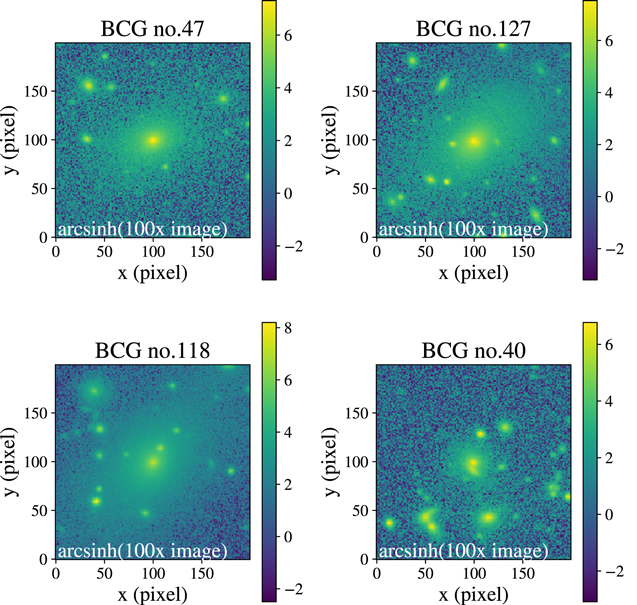
Figure 23. SDSS i-band images of the four notable BCGs as noted in Appendix B.1, zoomed in to the central 200 pixels.
Download figure:
Standard image High-resolution imageB.1. Notable BCGs in the Main Sample
First, two of the BCGs (Nos. 47 and 127) could have their brightest peak also detected as a core, because there are two nearly equally bright peaks at its center, and the SDSS pipeline sets the galaxy center in between the peaks. For these objects, we update the position of BCG to the brightest peak and apply our detection relative to this new position.
Second, the spaxels of the core of BCG No. 118 are mostly masked out in DAP in MPL-9 but partially retained in MPL-6. Hence, we use the MPL-6 map for this source (see Figure 24).
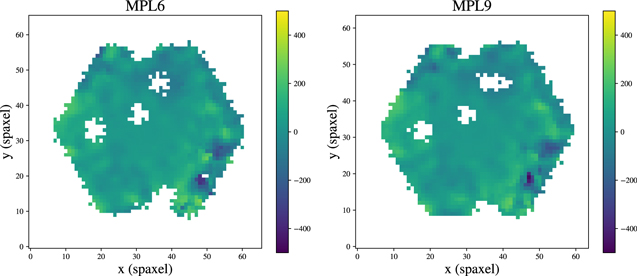
Figure 24. MPL-6 and MPL-9 MaNGA stellar velocity map with "DONOTUSE" mask applied, for BCG No. 118.
Download figure:
Standard image High-resolution imageThird, the IFU observation of BCG No. 40 is targeting a satellite instead of the BCG. This is because the target belongs to a MaNGA ancillary program investigating close pairs and mergers (Wake et al. 2017), whose targets are selected from the NSA catalog with a velocity difference of less than 500 km s−1. Therefore, although we cannot measure its velocity difference relative to the BCG main body, it still satisfies our criteria.
Finally, recall that, we mainly use the 800 × 800 pixel images and their BACK_SIZE = 160 (1/5 image size) segmentation maps for our BCGs. The 1000 × 1000 pixel image and the BACK_SIZE = 160 (1/3 image size) set is used in a few cases (4 out of 89 in the Main sample) when the segmentation and Ellipse models of the two versions are different, and we prefer the 1000 × 1000 pixel version. The 800 × 800 image and the BACK_SIZE = 160 (1/3 image size) are used for BCG No. 68; however, because the usual settings cannot mask out a bright elongated galaxy in its image.
B.2. Notable BCGs in TNG300
There are two objects in the TNG sample that the single Sérsic fit fails, and we use the Ellipse total flux within 150 kpc instead (Figure 25).
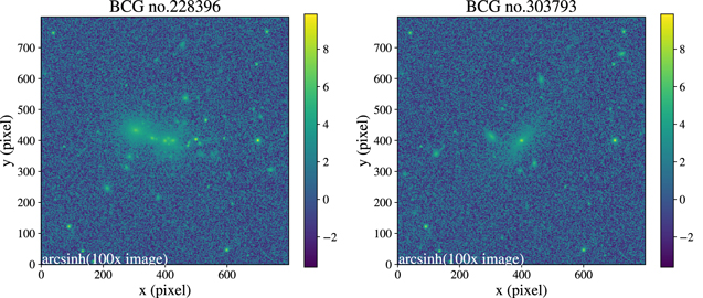
Figure 25. Images of the two notable BCGs in TNG300.
Download figure:
Standard image High-resolution imageThe BCG of halo 228396 consists of four blending bright objects, and this complex morphology causes a single Sérsic fit to fail. We still use the Ellipse photometry because, even though the curve of growth of the primary object is strongly affected by the other objects, they are all considered as the components of the BCG.
The BCG of halo 303793 has an unusual morphology that has a bright core in the center and a faint and very elongated outskirt. As the light is very concentrated and the Sérsic fit fails, we use the flux within 150 kpc.
B.3. Changed BCGs
In the BCG identification process, we have changed five BCGs originally identified by Y07 to another galaxy. The SDSS images of the original BCGs in Y07 and the new BCGs are shown in Figure 26. The color–magnitude diagrams of these clusters are shown in Figures 27 and 28. BCGs Nos. 23, 35, 52, 68 are changed because they are spiral galaxies. BCG No. 62 is not the most luminous galaxy within a projected distance of 800 kpc from the cluster center, so we select the truly most luminous one as the BCG, 36 where the luminosity is taken from the NSA catalog. Among the changed galaxies, Nos. 52, 62, 68 are in our Main sample (please see Appendix B.4.1 below for more details). As can be seen from Figure 26, the original BCG of cluster No. 62 has a core; using MaNGA velocity map we have measured a velocity offset of −286 km s−1. Had we adopted it as the BCG, our multiple-core frequency would increase slightly from 0.11 ± 0.04 to 0.13 ± 0.04.
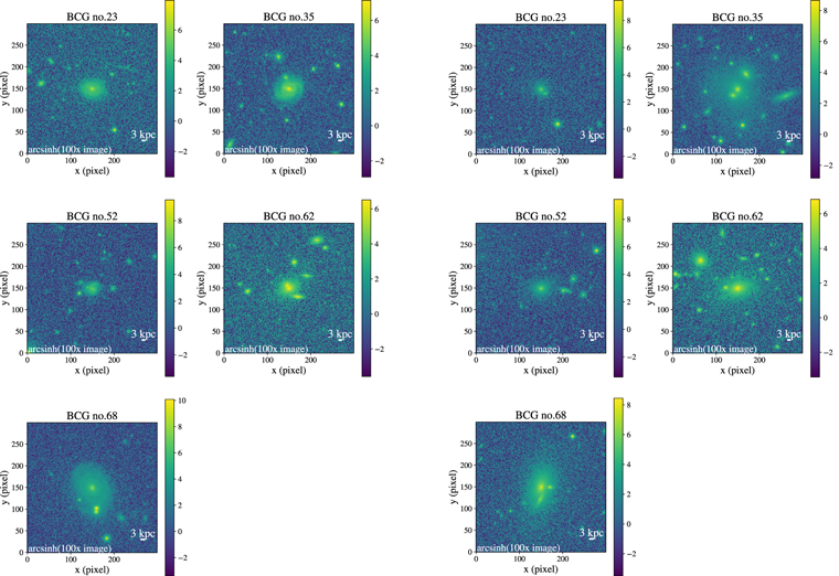
Figure 26. Left: The SDSS images of the 5 Y07 BCGs that are changed during our BCG identification process, zoomed in to the central 300 pixels. It can be noticed that there is a core in BCG No. 62; it has a velocity offset of −286 km s−1. Adopting this galaxy as the BCG would change our fmc to 0.13 ± 0.04. Right: The images of the five BCGs identified by us, zoomed in to the central 300 pixels.
Download figure:
Standard image High-resolution image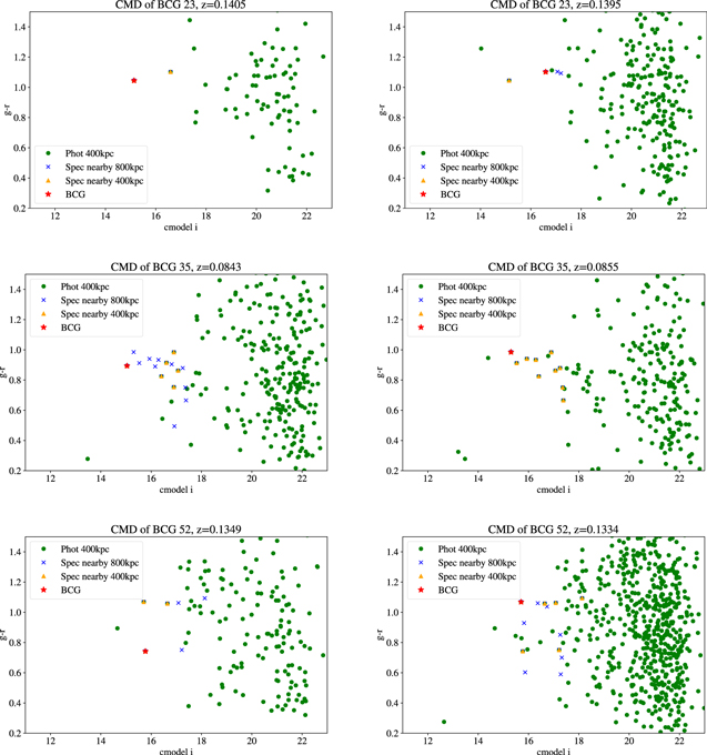
Figure 27. Left: Color–magnitude diagrams (CMDs) of three Y07 BCGs (Nos. 23, 35, and 52) that are changed in our BGC identification process. The color is extinction corrected model g − r magnitude, and the x-axis is the cmodel (de Vaucouleurs+Exponential) i-band magnitude. The red star represents the BCG. The green dots are the SDSS galaxies within a 400 kpc radius. The blue crosses are the SDSS galaxies with spectroscopy within 800 kpc radius and redshift offset <0.01. The yellow triangles are SDSS galaxies with spectroscopy within a 400 kpc radius. Right: CMDs showing the location of our chosen BCGs.
Download figure:
Standard image High-resolution image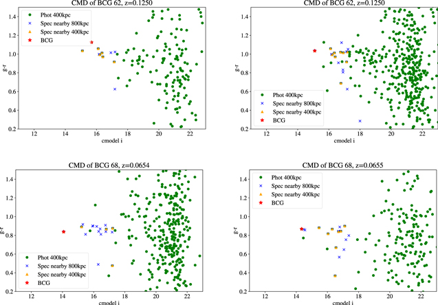
Figure 28. Same as Figure 27, but for BCGs Nos. 62 and 68.
Download figure:
Standard image High-resolution imageB.4. Excluded BCGs
B.4.1. Excluded Objects in the MPL-9 sample at the BCG Identification Stage
Seven objects are excluded in the BCG identification process (Figure 29). BCG No. 15 has only few neighbors that can be seen in the SDSS image, and a few spectroscopically confirmed members (Figure 30, right panel) in the cluster catalog. Also, its red sequence is not obvious (left panel). BCGs Nos. 14, 37, 58 have a spiral morphology, and we could not find other BCG candidates for their host clusters. BCGs Nos. 23 and 35 are chosen based on our selection criteria (see Appendix B.3), but they are not observed by MaNGA. The BCG of the Coma cluster (No. 126) is also excluded not only because it is very nearby and resolved, but also because it is observed by the Coma ancillary program and the DAP product does not include the maps of the BCG.
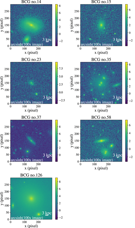
Figure 29. SDSS images of the seven BCGs removed during our BCG identification process, zoomed in to the central 300 pixels. Note that for Nos. 23 and 35 it is the BCG that we have chosen, not the one from the Y07 catalog.
Download figure:
Standard image High-resolution image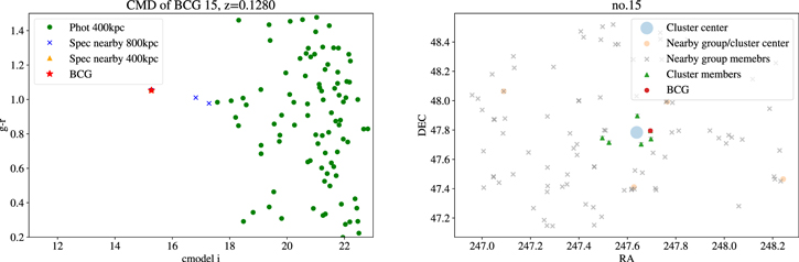
Figure 30. Left: Color–magnitude diagram (CMD) of BCG No. 15. The color is extinction corrected model g − r magnitude, while the x-axis is the cmodel (de Vaucouleurs+Exponential) i-band magnitude. The red star represents the BCG. The green dots are the SDSS galaxies within a 400 kpc radius. The blue crosses are the SDSS galaxies with spectroscopy within an 800 kpc radius and redshift offset < 0.01. The are no SDSS galaxies with spectroscopy within a 400 kpc radius (yellow triangle). Right: The spatial distribution member galaxies of the cluster that hosts BCG No. 15. The red dot represents the BCG identified by the Y07 catalog. The blue circle is the center of the cluster. The green triangles are the spectroscopically confirmed cluster members. The gray crosses (yellow circles) are the other galaxies (clusters) in the Y07 catalog that are within 075 radius and redshift offset < 0.1.
Download figure:
Standard image High-resolution imageB.4.2. Excluded Objects in the MPL-9 Sample Due to Image Quality Issues
Six BCGs are excluded due to the image quality issues. As shown in Figure 31 (left panel), BCG Nos. 63, 75, and 100 have artificial features across the BCG. BCG Nos. 75, 85, 87, 92 have bright stars close to the BCG. These can cause problems in background subtraction and affect the resulting Ellipse models.
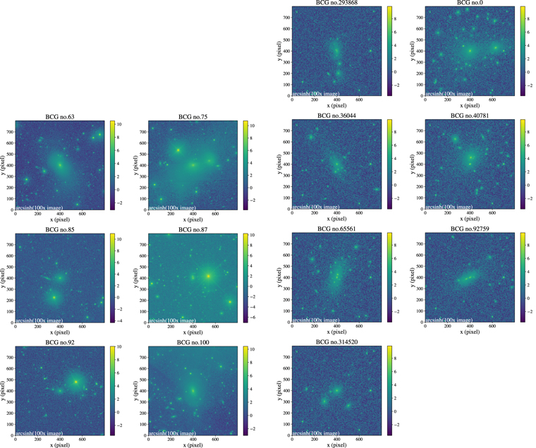
Figure 31. Left: SDSS i-band images of the six BCGs that are excluded due to image quality issues. Right: Images of the seven simulated BCGs that are excluded.
Download figure:
Standard image High-resolution imageB.4.3. Excluded BCGs in TNG300
Seven BCGs are excluded in the simulated sample, because their morphologies are too complex and we cannot obtain a reliable total flux (Figure 31, right panel). We emphasize that no such problems occur for the real BCGs in our Main sample. However, mergers might be related to the complex morphology, so we present two multiple-core frequencies in the main text, one including and the other excluding these objects (Section 4.6).
The BCG of halo 293868 has many small neighbors touching it, and its Ellipse surface brightness profile is nonmonotonic and is unreliable, forcing us to exclude it. This object (and its host halo) is the one that we remove in Section 4.1.
The BCG of halo 0 has a bright neighbor in the field of view and the outskirt light of the neighbor affects the outskirt of the curve of growth. Also, the mass of this halo is 1.2 × 10¹⁵ h−1 M⊙, far exceeding the massive end of our Main sample.
The BCG of halo 36044 also has many small neighbors touching it and the blending affects the curve of growth at the outskirt. Its Re of the single Sérsic fit is larger than 500'', which is unreliable large.
The BCG of halo 40781 also has many small neighbors touching it and the masking causes some dips in the Ellipse curve of growth and in turn, the single Sérsic fit failed.
The BCG of halo 65561 has a complex morphology that not only has many small neighbors touching it, and the center part consists of two cores with comparable brightness. This leads to a nonmonotonic surface brightness profile and unreasonable curve of growth; hence the single Sérsic fit fails.
The BCG of halo 92759 has bright neighbors touching it, and the blending affects the curve of growth. Its Re of the single Sérsic fit is larger than 700'', which is unreasonably large.
The BCG of halo 314520 has a bright neighbor in the field of view, and the outskirt light of the neighbor affects the outer parts of the curve of growth. Its Re of the single Sérsic fit is larger than 100''.
Footnotes
- 22
Using the version based on the Petrosian magnitude would affect the BCG selection at less than 1% level (X. Yang 2022, private communication).
- 23
- 24
- 25
- 26
Detection threshold = 0.2, minimum area = 1, deblend threshold = 64, deblend contrast = 0.0001, clean parameter = 1.0.
- 27
- 28
We caution that this choice depends on the cluster velocity dispersion; for the clusters in our sample, which have mass about 1014 M⊙, this is adequate.
- 29
f mc = (80.5 + 31.5 + 43.2)/1359 = 0.114.
- 30
The object has ID 293868 (see Appendix B.4.3). The reason for its removal is due to the difficulty of obtaining a good Ellipse model for it (see Section 4.3). As Re is necessary for our further analyses, and such a failure (which is not due to the presence of cores in the BCG) should be independent of its multiple-core frequency, removing this BCG from the sample should not affect our results.
- 31
Detection threshold = 0.2, minimum area = 1, deblend threshold = 64, deblend contrast = 0.0001, clean parameter = 1.0.
- 32
- 33
- 34
- 35
- 36
The reason for this is that additional redshifts from SDSS-III (Eisenstein et al. 2011) became available after the construction of the Y07 catalog. We note that this only occurs to this particular cluster; for all other clusters, the new redshifts from SDSS-III do not play a role in the choice of BCGs.