Abstract
Spiking neural networks (SNNs) have recently emerged as the low-power alternative to artificial neural networks (ANNs) because of their sparse, asynchronous, and binary event-driven processing. Due to their energy efficiency, SNNs have a high possibility of being deployed for real-world, resource-constrained systems such as autonomous vehicles and drones. However, owing to their non-differentiable and complex neuronal dynamics, most previous SNN optimization methods have been limited to image recognition. In this paper, we explore the SNN applications beyond classification and present semantic segmentation networks configured with spiking neurons. Specifically, we first investigate two representative SNN optimization techniques for recognition tasks (i.e., ANN-SNN conversion and surrogate gradient learning) on semantic segmentation datasets. We observe that, when converted from ANNs, SNNs suffer from high latency and low performance due to the spatial variance of features. Therefore, we directly train networks with surrogate gradient learning, resulting in lower latency and higher performance than ANN-SNN conversion. Moreover, we redesign two fundamental ANN segmentation architectures (i.e., Fully Convolutional Networks and DeepLab) for the SNN domain. We conduct experiments on three semantic segmentation benchmarks including PASCAL VOC2012 dataset, DDD17 event-based dataset, and synthetic segmentation dataset combined CIFAR10 and MNIST datasets. In addition to showing the feasibility of SNNs for semantic segmentation, we show that SNNs can be more robust and energy-efficient compared to their ANN counterparts in this domain.
Export citation and abstract BibTeX RIS
Original content from this work may be used under the terms of the Creative Commons Attribution 4.0 licence. Any further distribution of this work must maintain attribution to the author(s) and the title of the work, journal citation and DOI.
1. Introduction
Artificial neural networks (ANNs) have shown impressive performance across various computer vision fields for a few decades [1–3]. However, ANNs suffer from huge computational costs [4], limiting their application in power-hungry systems such as internet-of-things (IoT) devices. As an alternative to low-power ANNs, recent studies have focused on bio-plausible spiking neural networks (SNNs) [5, 6], which process visual information with temporal binary events (i.e., spikes). Spikes stimulate neuronal membrane potentials and convey discriminative information from shallow layers to deep layers. SNN neurons only consume energy whenever spikes are generated which allow for these asynchronous processes to be implemented on highly energy-efficient neuromorphic hardware [7–9].
In order to exploit the energy advantage of binary information transmission, optimization algorithms for SNNs have been developed in the past few decades, with a focus on image classification. Among various training algorithms, the ANN-SNN conversion method [10–13] has been highlighted as a result of its simplicity and high performance. Conversion replaces the neurons of a pre-trained ANN using the ReLU activation function with integrate-and-fire (IF) neurons in an SNN. The conversion method avoids the complexity of spike-based training since it relies on ANN training and thus, yields high performance on complex data. However, since conversion naively scales the firing thresholds with the maximum layer activations, it is hard to capture spike information across the spatial and temporal domain. As a result, the SNN created using ANN-SNN conversion requires thousands of time-steps to achieve similar performance as the original pre-trained ANN, and has been limited to fundamental vision tasks such as image classification.
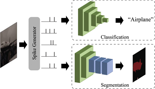
Considering the likelihood of the future deployment of SNNs in scene-understanding tasks, it is essential to investigate the applicability of SNNs for beyond classification. For example, a vision system for autonomous vehicles should contain an energy-efficient neural module for analyzing the overall context of scenery [14, 15]. Therefore, in this paper, we move beyond classification by exploring semantic segmentation for neuromorphic systems. As shown in figure 1, a semantic segmentation network conducts pixel-wise classification, resulting in a two-dimensional prediction map. Since partitioning multiple foreground objects from the background is an essential and fundamental vision task, semantic segmentation has been extensively studied in the ANN domain [1, 16–19]. Unfortunately, ANN-SNN conversion cannot be compatible with a spike stream dataset from dynamic vision sensor (DVS) camera [20–23], which limits the potential advantage of a neuromorphic system.
Figure 1. The concept of image classification and semantic segmentation. For a given image, the classification network provides a class prediction (e.g., airplane). On the other hand, the semantic segmentation network maintains the high resolution feature map at the end of the network (colored in blue) and assigns every pixel in the image its own class, resulting in a two-dimensional prediction map.
Download figure:
Standard image High-resolution imageTo address the aforementioned problems, we focus on surrogate gradient backpropagation learning [24–26] rather than ANN-SNN conversion, which directly trains SNNs from input spikes. The major difficulty of gradient backpropagation learning with SNNs is the non-differentiable neuronal functionality of SNNs. A leaky integrate-and-fire (LIF) neuron does not generate spikes before its membrane potential exceeds a firing threshold, resulting in a non-differentiable point during backpropagation. Therefore, we approximate the backward gradient function of an LIF neuron using a piece-wise linear function during backpropagation. Using the approximated gradient function, the weight parameters are optimized in order to minimize spatial cross-entropy loss. In addition, we leverage batch normalization through time (BNTT) [27], a recent work proposes a temporal batch normalization, which enables our segmentation networks to be trained from scratch. As a result, SNNs with BNTT-backpropagation can learn the temporal dynamics of input spikes, with shorter number of time-steps and better performance compared to ANN-SNN conversion.
With surrogate learning, we investigate two representative segmentation architectures from the ANN domain, i.e., fully convolutional networks (FCNs) [19] and DeepLab with dilated (i.e., atrous) convolutional layers [1]. The FCN architecture consists of an encoder-decoder architecture, which recovers the resolution of the original image with the upsampling decoder. On the other hand, DeepLab only has an encoder architecture but uses dilated convolutions to cover wide receptive fields without computational overhead. Due to the fact that very deep SNN architectures suffer performance degradation because of the mismatch between real gradients and approximated gradients, we use the VGG9 architecture as the backbone for our networks for segmentation.
In summary, the main contributions of this work are as follows: (i) to the best of our knowledge, our work is the first work to train SNNs for semantic segmentation. This is an important research direction given that low-power SNNs will be deployed in scene-understanding tasks. (ii) We investigate two representative SNN optimization techniques (e.g., ANN-SNN conversion and surrogate gradient learning) on semantic segmentation datasets. We observe that surrogate gradient learning achieves better performance with lower latency compared to ANN-SNN conversion. (iii) We present spiking-FCN and Spiking-DeepLab, which expand upon the two fundamental architectures used for semantic segmentation in the ANN domain. Also, we conduct comprehensive experiments on various benchmarks including static PASCAL VOC2012, DDD17 from a DVS camera, and synthetic MNIST-CIFAR10-segmentation dataset. The proposed segmentation architectures can bring a more than 2× energy efficiency than standard ANNs.
The paper is organized as follows. Section 2 introduces background knowledge on SNNs and the semantic segmentation work done in the ANN domain. Section 3 presents our experiments on ANN-SNN conversion. Section 4 details our methods of training segmentation networks with spiking neurons. Lastly, in section 5, we present our comprehensive experimental results on both the static and video segmentation datasets. At the end of this paper, we provide our conclusions and point out future work directions.
2. Related work
2.1. Spiking neural network
Spiking neural networks (SNNs) have emerged as the next generation of neural networks [5, 28–34], because they offer huge energy-efficiency advantage over ANNs. Different from standard ANNs that make use of float values, SNNs process binary spikes (0 or 1) across multiple time-steps. SNNs take binary spike trains as an input, which can be obtained from both static RGB images and DVS camera data. For static images, various coding schemes have been proposed. Poisson rate coding generates spikes in which the number of spikes is proportional to the pixel intensity. Due to its simplicity and high performance, Poisson rate coding has been widely used in previous works [5, 25, 30]. Temporal coding allows only one spike per neuron, resulting in energy efficiency from fewer spikes. Here, spike latency is inversely proportional to the pixel intensity [31, 35, 36]. Thus, bright pixels generate more spike events in earlier time-steps than dark pixels. However, for DVS camera data, SNNs can be directly trained without any code generator.
In terms of an activation function, SNNs commonly use a leaky integrate-and-fire (LIF) neuron [37]. The LIF neuron (figure 2) has a membrane potential which can store the temporal information by accumulating pre-synaptic spikes. The neuron generates a post-synaptic spike whenever the membrane potential exceeds a predefined firing threshold. This integrate-and-fire behavior is non-differentiable, so SNNs are hard to train with standard backpropagation [24]. To address this limitation, work in the past decade has focused on various training techniques for SNNs. Spike-timing-dependent plasticity (STDP) learning [38–40] is based on the neuroscience observation that weight connections can be reinforced or punished according to the temporal correlation of spikes. STDP learning can be implemented without a complicated backpropagation module but can only be applied to small-scale tasks due to its locality [41, 42]. ANN-SNN conversion methods have received attention due to their high performance on complex tasks [10–13]. In order to approximate ReLU activations with LIF activations, pre-trained ANNs are converted to SNNs using weight (or threshold) balancing techniques. ANN-SNN conversion requires many time-steps to represent the float values of ANNs with binary spikes. Surrogate gradient learning addresses the non-differentiability of LIF neurons by defining a surrogate gradient function in a backpropagation process [24, 25]. This training scheme enables SNNs to learn the temporal dynamics of spike trains, resulting in small latency and reasonable performance. Unfortunately, most SNN optimization algorithms are developed for basic, fundamental vision tasks such as image recognition [25, 27, 30], visualization [43], and optimization [44, 45].
Figure 2. The neuronal dynamics of SNNs. Pre-synaptic neurons convey spike trains to a post-synaptic neuron. This increases the membrane potential voltage and the post-synaptic neuron generates the output spikes whenever the membrane potential exceeds the neuronal firing threshold. After that, the membrane potential is set to a reset voltage.
Download figure:
Standard image High-resolution image2.2. Semantic segmentation
The objective of semantic segmentation is to classify every pixel in an image with a label, a key task for scene understanding. This becomes more important with the development of medical image analysis [47, 48], autonomous vehicles [15, 49], and augmented reality [50]. Therefore, semantic segmentation with deep neural networks has been extensively studied in the ANN domain. The fully convolutional network (FCN) [19] is the one of the pioneering works in deep semantic segmentation. FCNs preserve image details by adding the intermediate high-resolution feature maps into its decoder path. In a similar way, U-Net [47] concatenates intermediate feature maps during its up-convolution process. Different from previous approaches, deconvolution networks [51] do not exploit a skip connection but learn a detailed representation from low-resolution feature maps. RefineNet [52] uses multi-scale inputs in order to enhance detail in the segmentation map. DeepLab [1] utilizes dilated (i.e., atrous) convolutions which enlarge the receptive field without any additional computational cost. Dilated convolutions have become one of the most popular techniques for semantic segmentation since they are easy to be implemented in deep learning frameworks (e.g., TensorFlow [53]). Despite its importance and fast growth in the ANN domain, semantic segmentation has not yet been studied with spiking neurons. So far, in the SNN domain, a few works [54, 55] have proposed region segmentation without providing semantic information (i.e., class information). Also, although a line of works [56, 57] have proposed foreground/background segmentation using modified STDP learning rules, large-scale multi-class semantic segmentation is still missing. In order to fill the gap, in this work, we configure the spiking versions of segmentation networks based on two representative segmentation architectures, i.e., FCN and DeepLab.
2.3. Novel SNN hardware architecture
Although the primary neuromorphic hardware like Loihi, TrueNorth, and SpiNNaker [7–9] provide huge energy-efficiency on small-scale optimization tasks, they cannot achieve better efficiency compared to the traditional CPUs and GPUs (e.g., Nvidia GPUs and Intel Xeon CPUs) on large-scale image classification tasks [58]. To address this, a line of works has proposed von-Neumann SNN hardware architectures. Parallel-time batching (PTB) [59] presents a modified dataflow for data reuse in temporal batch-processing, resulting in the significant energy efficiency of SNNs by 198× compared to a baseline without PTB. Recently, Narayanan et al [60] find that rate-coded SNNs bring high computational costs on traditional von-Neumann architectures. To mitigate this, they introduce spiking-Eyeriss architecture with temporal-coded SNNs, achieving higher energy efficiency than rate-coded SNNs.
Recent SNN hardware architectures also leverage in-memory computing architecture where they conduct calculations inside the memory. The in-memory computing architecture does not suffer from high memory energy overhead and lower computation bandwidth in traditional von-Neumann architectures. Ankit et al [61] utilize analog crossbar architectures and present SNNs can achieve 900× reduction in energy-delay product (EDP) compared to CMOS von-Neumann accelerators while preserving classification accuracy.
Interestingly, recent work [62] presents sparsity-aware digital hardware for a segmentation task with SNNs. They design a reconfigurable spiking neural processing unit that dynamically skips zero values, resulting in 65uJ energy consumption at 2.2k FPS with TSMC 28 nm technology. We expect that their hardware will provide positive synergy with our segmentation model since our model has a low spike rate (shown in section 5) and similar network architecture (encoder-decoder) as [63].
3. Preliminary study
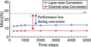
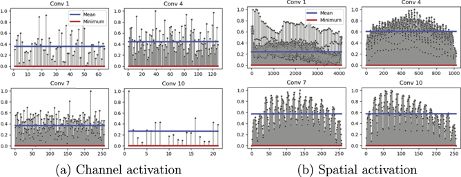
In this section, we apply ANN-SNN conversion methods to semantic segmentation. First, we train the ANN-DeepLab with conventional 2D-cross entropy loss [1]. After that, we convert the pre-trained ANN to an SNN with two conversion methods [10, 46]. Sengputa et al [10] propose a state-of-the-art conversion technique in the image recognition domain. They take into account spike behavior in the previous layers to achieve accurate weight balancing. Also, the authors of [46] propose channel-wise weight balancing for each layer in order to capture a feature with high variation in an object detection scenario. We evaluate these methods on a DeepLab architecture with a VGG9 backbone network [63] on PASCAL VOC2012 dataset [64]. In figure 3, we observe that the ANN-SNN conversion process significantly degrades the performance from a pre-trained ANN even with thousands of time-steps. This is a relatively huge loss compared to ANN-SNN conversion on image classification which shows less than 1% accuracy degradation [10]. The reason for this is that networks trained for the semantic segmentation task have a large variation of activations in both the channel and spatial axes (figure 4). This causes ANN-SNN conversion to fail to find a proper scaling factor. Thus, applying the same balancing factor across layers (or channels) does not fully preserve delicate activations. Note, it is interesting that layer-wise conversion shows higher performance than channel-wise conversion. If we apply channel-wise ANN-SNN conversion, the channel features will have more discriminative representation than the spatial feature. As the feature goes through layers, the channel features might largely affect the final prediction. We conjecture this deteriorates segmentation performance where capturing detailed spatial boundaries is important. More importantly, ANN-SNN conversion cannot be applied on video spike streams from a DVS camera, since ANN-SNN conversion is only compatible with static images. Thus, we focus on a direct training approach in order to implement semantic segmentation with spiking neurons.
Figure 3. Performance of converted SNNs with respect to the number of time-steps. We evaluate two conversion algorithms (i.e., layer-wise conversion [10] and channel-wise conversion [46]) with a DeepLab architecture trained on PASCAL VOC2012. Compared to the ANN performance (black dotted line), the converted SNNs suffer from performance degradation caused by a large variation in activations.
Download figure:
Standard image High-resolution imageFigure 4. Illustration of normalized maximum activations across (a) channel and (b) spatial axes. We use a VGG9-based DeepLab architecture trained on PASCAL VOC2012 dataset. In the figure, the x and y axes denote, respectively, the index of the channel/spatial axes in that layer and the normalized maximum activations across the channel/spatial axes.
Download figure:
Standard image High-resolution image4. Methodology
4.1. Leaky integrate-and-fire (LIF) neuron
We leverage a leaky integrate-and-fire (LIF) neuron in our spiking segmentation networks. Figure 2 illustrates the dynamics of an LIF neuron. The LIF neuron can be represented with a membrane potential and an input signal. The membrane potential Um stores the temporal spike information in capacitance. When an input signal I(t) is fed into the LIF neuron, the membrane potential is changed according to the following differential equation:

where, R is an input resistance for the LIF circuit and τm is the time constant for the membrane potential decay. Since the voltage and current have continuous values, we convert the differential equation into a discrete version in order to conduct digital simulation. We can represent the membrane potential  of a single neuron i at time-step t as:

Here, the current membrane potential consists of the decayed membrane potential from previous time-steps and the weighted spike signal from the pre-synaptic neurons j. The notation λ and wij
are for a leak factor and weight connection between the pre-synaptic neuron j and the post-synaptic neuron i, respectively. When  exceeds the firing threshold, the neuron i generates a spike output
  :
:

After the neuron fires, the membrane potential is lowered by the amount of the threshold (i.e., soft reset). In our experiments, we use a soft reset scheme since it achieves better performance than a hard reset (i.e., reset to the minimum voltage such as zero). This is because a soft reset allows the neuron to retain residual information after the reset, thus preventing information loss [11].
4.2. Input representation
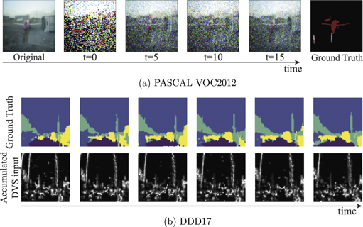
In this paper, we use two types of input datasets, i.e., static images and DVS data. For training and inference, a static image needs to be converted into spike trains since SNNs process multiple binary spikes. There are various spike coding schemes such as rate, temporal, and phase [35, 65]. Among them, we use rate coding due to its reliable performance across various tasks. Rate coding provides spikes proportional to the pixel intensity of the given image. In order to implement this, following previous work [5], we compare each pixel value with a random number ranging between [Imin, Imax] at every time-step. Here, Imin and Imax correspond to the minimum and maximum possible pixel intensities. If the random number is greater than the pixel intensity, the Poisson spike generator outputs a spike with amplitude 1. Otherwise, the Poisson spike generator does not yield any spikes. We visualize rate coding in figure 5(a). We see that the spikes generated at a given time-step is random. However, as time goes on, the accumulated spikes represent a similar result to the original image. For a DVS spike stream, we accumulate spikes in a certain time window to generate a frame. Then, the network processes these frames like a video input (figure 5(b)).
Figure 5. Examples of input representations. (a) We convert a static image into Poisson spikes. As time goes on, the accumulated spikes represent similar image to original image. (b) For the event-based camera input, we accumulate spikes in the pre-defined time window (e.g., 10 ms) to generate frames.
Download figure:
Standard image High-resolution image4.3. Spiking segmentation network architecture
4.3.1. Spiking-DeepLab
Different from image recognition tasks, segmentation networks provide pixel-wise classification with respect to the given two-dimensional input image. Therefore, the segmentation architecture needs to maintain a large spatial resolution of the feature maps at the end of the network. Also, taking a large receptive field helps the networks figure out the relationships between objects in the scene, resulting in high performance. To this end, DeepLab [63] proposed a dilated convolution in order to fulfill these two objectives. The dilated convolution puts space between the kernel weights. As a result, the dilated convolution operation increases the size of the receptive field without adding a memory burden.
With the LIF neuron model, for a neuron at (ix , iy ), we can reformulate the neuronal dynamics (equation (2)) with the dilated convolution operation:

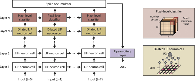
where, r is stride and K is kernel size. If we set r to 1, this equation is the same equation of a normal convolutional layer. If we increase the value of r, the receptive fields also increase proportional to r. For example, the area of a local receptive field with 3 × 3 kernel is 9. However, for a dilated convolutional layer with stride 2, the area of local receptive field increases to 25, as shown in the right bottom box in figure 6. We apply these dilated convolutional layers to the last two convolutional layers in the feature extractor.
Figure 6. Spiking-DeepLab: a computational graph unrolled over multiple time-steps. Each neuron cell has a membrane potential consisting of temporal voltage propagation (i.e., horizontal arrow) and the spikes from previous layer (i.e., vertical arrow). In order to increase the receptive field in deep layers, we add a dilated LIF neuron cell which can cover a larger spatial area with the same number of parameters. We apply dilated convolution layers for the last Convolution block following the original Deeplab architecture. For the last layer, we accumulate output spikes across all time-steps and generate a two-dimensional probabilistic map. Finally, we upsample the final prediction map to the original resolution of the input image and calculate the loss function to update the weights.
Download figure:
Standard image High-resolution imageFigure 6 illustrates the computational graph of spiking-DeepLab. According to equation (4), the membrane potential of each neuron is computed by combining the previous membrane potential (i.e., temporal propagation) and the previous layer (i.e., spatial propagation). To preserve the size of the feature map in deep layers, we do not apply average pooling layers in the last feature extraction block (architecture details are shown in table 1). Also, it is worth mentioning that we use a pixel-wise classifier at the last layer of the network, resulting in a tensor in which the channel size is the number of classes. We accumulate spikes at the last layer across all timesteps, and select the class corresponding to the maximum number of spikes at each pixel location.
Table 1. SNN architectures of DeepLab and FCN.
| Module | Spiking-DeepLab | Spiking-FCN |
|---|---|---|
| Conv [(3, 64), kernelsize = 3, stride = 1] | Conv [(64, 64), kernelsize = 3, stride = 1] | |
| Conv [(64, 64), kernelsize = 3, stride = 1] | Conv [(64, 64), kernelsize = 3, stride = 1] | |
| AvgPool [kernelsize = 3, stride 2] | AvgPool [kernelsize = 3, stride 2] | |
| Conv [(64, 128), kernelsize = 3, stride = 1] | Conv [(64, 128), kernelsize = 3, stride = 1] | |
| Downsampling layers | Conv [(128, 128), kernelsize = 3, stride = 1] | Conv [(128, 128), kernelsize = 3, stride = 1] |
| AvgPool [kernelsize = 3, stride 2] | AvgPool [kernelsize = 3, stride 2] | |
| Conv [(128, 256), kernelsize = 3, stride = 1] | Conv [(128, 256), kernelsize = 3, stride = 1] | |
| Dilated Conv [(256, 256), kernelsize = 3, stride = 1, dilation = 2] | Conv [(128, 256), kernelsize = 3, stride = 1] | |
| Conv [(256, 256), kernelsize = 3, stride = 1] | ||
| Dilated Conv [(256, 256), kernelsize = 3, stride = 1, dilation = 2] | Conv [(256, 256), kernelsize = 3, stride = 1] | |
| AvgPool [kernelsize = 3, stride 2] | ||
| Intermediate Layers | Dilated Conv [(256, 1024), kernelsize = 3, stride = 1, dilation = 12] | Conv [(256, 1024), kernelsize = 1, stride = 1] |
| Conv [Number of classes, kernelsize = 1, stride = 1] | Conv [(1024, 1024), kernelsize = 1, stride = 1] | |
| Conv [(1024, Number of classes), kernelsize = 3, stride = 2] | ||
| TransposeConv [Number of classes] | ||
| SkipConv [(256, Number of classes), kernelsize = 3, stride = 2] | ||
| Upsampling Layers | Bilinear interpolation | TransposeConv [Number of classes] |
| SkipConv [(128, Number of classes), kernelsize = 3, stride = 2] | ||
| TransposeConv [Number of classes] | ||
| SkipConv [(64, Number of classes), kernelsize = 3, stride = 2] |
4.3.2. Spiking fully-convolutional networks (FCN)
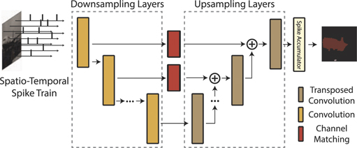
Another fundamental architecture for segmentation is fully-convolutional networks (FCN). Different from DeepLab where a high resolution feature map is maintained, FCN consists of a downsampling network and an upsampling network. The downsampling network discovers the semantic representation of the given input images. This is similar to image recognition networks which consist of multiple convolution and pooling layers. The upsampling network recovers the resolution of the small feature map by upsampling it into the original image resolution using transposed convolutional layers. The transposed convolutional layer increases the resolution of the input feature map to a desired output feature map size with learn-able kernel parameters. These parameters are also trained with gradient-based learning. While increasing the resolution, following the original FCN paper [19], we add intermediate features from the downsampling network to features from the upsampling network. Here, we use convolutional layers to match the number of channels between features in downsampling and upsampling. Note that all layers consist of LIF neurons, and thus features are processed in a temporal manner. In addition, like the DeepLab architecture, we use the spike accumulator at the end of the network. We visualize the architecture (not the computational graph) of FCN in figure 7. The computational graph of Spiking-FCN can be represented with a similar structure as spiking-DeepLab.
Figure 7. An illustration of the FCN architecture.
Download figure:
Standard image High-resolution image4.4. Overall optimization
For both architectures, the network provides a two-dimensional probabilistic map at the output layer. This probabilistic map is based on the stacked spike voltage from the spike accumulator. For every pixel location (p, q), with the given ground truth label yi , we compute the cross-entropy loss as:

Here, N and C represent a normalization factor and the number of classes, respectively. Also, hk stands for the number of accumulated spikes of the neurons in the last layer. We calculate backward gradients based on this spatial cross-entropy loss.
Backward gradients are computed based on surrogate back-propagation through time (BPTT) [24, 26] in which gradients are accumulated over all time-steps across all layers. For a hidden layer, the gradient of output spikes with respect to a membrane potential (i.e.,  ) is not differentiable because of the firing behavior of the LIF neuron (figure 2). To enable backpropagation through multiple layers, we approximate the backward gradient function to a piece-wise linear function:

For the last layer (i.e., classifier), weight parameters can be updated by conventional gradient backpropagation since we accumulate the spikes and conduct a single forward step in the last layer. Overall, weight parameters are updated based on the accumulated gradients at each layer. The accumulated gradients of loss L with respect to weights Wl at layer l can be calculated as:

Here, Ol and Ul stand for the output spike matrix and membrane potential matrix at layer l, respectively. We refer to [26] for more spatio-temporal backpropagation details. Algorithm 1 shows the overall optimization process of spiking segmentation networks with surrogate gradient backpropagation.
Algorithm 1. Directly training a segmentation network with surrogate gradient backpropagation.
| Input: SNN model (F), spike time-step (T); mini batch (X); labels (Y) | |
| Output: spiking segmentation network | |
| 1: for i ← 1 to max_iter do | |
| 2: fetch a mini batch X | |
| 3: for t ← 1 to T do | |
4:  PoissonGenerator(X) (or DVS input X) PoissonGenerator(X) (or DVS input X) | |
| 5: for l ← 1 to L − 1 do | |
6: 
| ⊳ Equation (4) |
| 7: end for | |
8: 
| ⊳ Final layer |
| 9: end for | |
10: 
| |
| 11: Do back-propagation and weight update | |
| 12: end for |
5. Experiments
5.1. Experimental setup
5.1.1. Dataset
We evaluate our methods on two semantic segmentation datasets: PASCAL VOC2012 and DDD17.
PASCAL VOC2012 [64] contains static images taken with a conventional camera classified with 20 foreground object classes and one background class. We use an augmented dataset [66] consisting of a training split of 10 582 images and a validation split of 1449 images. We re-scale the various original image resolutions to 64 × 64 pixels. For SNN models trained and evaluated on PASCAL VOC2012, we use a rate coding technique (discussed in section 4.2). Note, we use PASCAL VOC2012 and VOC2012 interchangeably in the remainder of the paper.
DDD17 [67] contains 40 different driving sequences of event data captured by a DVS camera. While the dataset provides both grayscale images and event data, it does not provide semantic segmentation labels. Therefore, we use the segmentation labels provided in [68], which consists of 20 different sequence intervals in 6 of the original DDD17 sequences. From these sequence intervals, we use a training split consisting of 15 950 frames and a testing split consisting of 3890 frames with 6 classes. We use a two-channel event representation of accumulated positive and negative events (integrated for a time interval of 50 ms) from the DVS dataset proposed in [68], and we re-scale the image resolution of 346 × 200 pixels to 64 × 64 pixels. In order to train SNNs with DDD17, we do not apply the Poisson coding technique since DDD17 contains temporally-related sequential samples. Therefore, we construct a batch with multiple sequences of successive video frames to leverage temporal information. Also, the prediction of an SNN model is based on the previous T video frames. For ANNs, we give each frames to networks, and average all embedding features (after the feature extractor) in temporal axis.
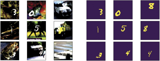
MNIST-CIFAR10-Segmentation. We use the simple segmentation dataset generation method [69] where the images consist of CIFAR10 background and MNIST foreground. The objective here is to segment the digit region from the whole picture. In figure 8, we visualize the generated images and the corresponding ground truth. We generate 48 000 training samples 12 000 test samples.
Figure 8. Synthetic segmentation dataset where the foreground is sampled by MNIST and background is sampled by CIFAR10.
Download figure:
Standard image High-resolution image5.1.2. Parameters
In our experiments, we use two different types of SNNs as shown in table 1. For both networks, the backbone network consists of 7 layers since it is difficult to increase depth with SNNs due to the real vs surrogate gradient discrepancy. Note that the main advantage of SNNs is huge energy efficiency compared to ANN, which is desirable for artificial Intelligence systems in edge devices. A Spiking-DeepLab model includes two dilated convolutional layers in the backbone network followed by a three-layer classifier. For Spiking-DeepLab, we use bilinear interpolation to upsample the output prediction to a segmentation map. Our Spiking-FCN model is similar to our Spiking-DeepLab model but does not use dilated convolutions and uses transposed convolutional layers for upsampling. SkipConv denotes the skip connection with channel reduction (red block in figure 7). We configure the same ANN architectures for comparison. In the ANNs, we use batch normalization [70] at each convolutional layer. For SNNs, we use the temporal batch normalization through time (BNTT) technique [27].
We train both networks using the same hyperparameters. We use an Adam optimizer with learning rate 3 × 10⁻³. We use a batch size of 16. Also, we use step-wise learning rate scheduling with a decay factor of 10 at 50% of the total number of epochs. Here, we set the total number of epochs to 60. We set 20 time-steps, set a leak factor of 0.99, and use a membrane threshold of 1.0.
5.2. Performance comparison
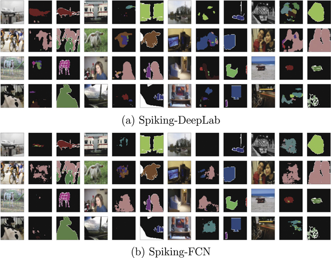
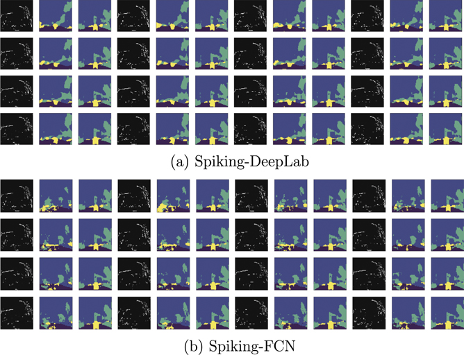
On public datasets, we compare the proposed Spiking-DeepLab and Spiking-FCN methods with the reference ANN methods [1, 19]. In table 2, for our BNTT-surrogate gradient-based approaches, the Spiking-FCN architecture shows less performance than the Spiking-DeepLab counterpart on VOC2012. Also earlier works have shown that training SNNs with deeper architectures is more challenging than with shallower architectures [27, 28]. In contrast, the Spiking-FCN architecture showed similar performance to the Spiking-DeepLab on DDD17 and MNIST-CIFAR10-segmentation dataset, as shown in tables 3 and 4. Overall, across all datasets, ANN references have a higher performance than SNNs since they are based on a well-established training method. It is worth mentioning that our purpose is to expand the application of SNNs and show the feasibility of various training methods. In the following sections, we show SNNs have the advantages of robustness and energy-efficiency. We also visualize the segmentation results on both datasets in figures 9 and 10.
Table 2. Mean IoU (%) of ANNs, spiking-FCN, and spiking-DeepLab on PASCAL VOC2012.
| Method | Time-steps | MIoU(%) |
|---|---|---|
| DeepLab [63] | — | 34.7 |
| FCN [19] | — | 32.9 |
| Spiking-DeepLab (ours) | 20 | 22.3 |
| Spiking-FCN (ours) | 20 | 9.9 |
Table 3. Mean IoU (%) of ANNs, spiking-FCN, and spiking-DeepLab on DDD17.
| Method | Time-steps | MIoU(%) |
|---|---|---|
| DeepLab [63] | — | 34.1 |
| FCN [19] | — | 42.2 |
| Spiking-DeepLab (ours) | 20 | 33.7 |
| Spiking-FCN (ours) | 20 | 34.2 |
Table 4. Mean IoU (%) of ANNs and spiking-DeepLab on MNIST-CIFAR10-segmentation dataset.
| Method | Time-steps | MIoU(%) |
|---|---|---|
| DeepLab [63] | — | 73.56 |
| FCN [19] | — | 74.43 |
| Spiking-DeepLab (ours) | 20 | 65.31 |
| Spiking-FCN (ours) | 20 | 66.20 |
Figure 9. Qualitative results of Spiking-DeepLab and Spiking-FCN on the PASCAL VOC2012 validation set. We visualize the image-prediction-groundtruth triplet for each sample.
Download figure:
Standard image High-resolution imageFigure 10. Qualitative results of Spiking-DeepLab and Spiking-FCN on the DDD17 test set. We visualize the image-prediction-groundtruth triplet for each sample.
Download figure:
Standard image High-resolution image5.3. Analysis on the number of timesteps
We analyze the accuracy change of a SNN model with respect to the number of timesteps. Here, we first consider changing timesteps for both training and inference. We vary T = [10, 15, 20, 25, 30, 35, 40]. As shown in figure 12, there is a clear trade-off between timesteps and accuracy. For instance, the small number of timesteps (T = 10) only can achieve mIoU 8.44%, on the other hand, timestep 40 can achieve mIoU 27.91%. Also, the accuracy is saturated at around T = 30.
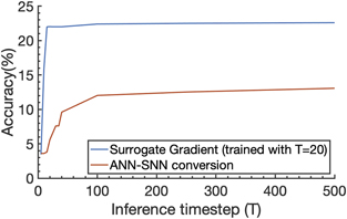
Moreover, we also shows the performance of trained SNN with T = 20, and test the model on different inference timesteps. After training a Spiking-DeepLab model with timestep 20, we measure the accuracy on timestep [5, 10, 15, 20, 25, 30, 35, 40, 100, 250, 500]. We plot the performance of Spiking-DeepLab and converted-DeepLab in figure 13. The results show that the accuracy of Spiking-DeepLab becomes saturated at T = 20 since we use T = 20 during training. The converted-DeepLab requires longer timesteps for reaching saturated performance. Also, the saturated performance of Spiking-DeepLab is higher than the converted-DeepLab.
5.4. Analysis on robustness
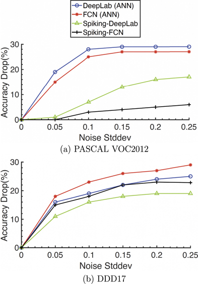
In real-world applications such as a self-driving vehicle, input signals are likely to be susceptible to noise. To investigate the effect of SNNs on robustness for segmentation, we evaluate the relative accuracy drop  in MIoU across varying levels of noise. Here, CleanMIoU and NoiseMIoU denote model MIoU when given clean samples and noisy samples, respectively. We add Gaussian noise (0, σ) to our inputs to generate noisy inputs. From figure 11(a), we observe that our SNNs (i.e., Spiking-DeepLab and Spiking-FCN) are more robust than ANNs for segmentation on VOC2012. This is because the Poisson spike generator converts a static pixel value into multiple temporal spikes with random distribution. From figure 11(b), we observe that SNNs show a similar robustness with ANNs on DDD17. Thus, SNNs trained on DDD17 (i.e., DVS event stream data) are less robust than SNNs trained on VOC2012 (i.e., static image). The main two factors contributing to this decrease in robustness are the following: (i) as aforementioned, the SNNs trained and evaluated on DDD17 do not use the Poisson coding technique which greatly affects robustness. (ii) The predictions of SNNs on DDD17 are based on multiple sequential frames whereas ANNs are only fed one input for each prediction. Therefore, more noise is accumulated across multiple frames for SNNs. However, despite the reduced robustness for segmentation on DVS data, segmentation networks with spiking neurons offer improved robustness for segmentation using traditional cameras.
Figure 11. Comparison of changes in mean IoU with respect to varying standard deviations of Gaussian noise. We use relative accuracy drop  where CleanMIoU and NoiseMIoU denote MIoU with clean and noise samples, respectively. The lower the relative accuracy drop is, the more robust the model is at that noise level.
Download figure:
Standard image High-resolution imageFigure 12. The trade-off between accuracy and timesteps of Spiking-SNN. We use the VOC2012 dataset with VGG9 architecture.
Download figure:
Standard image High-resolution imageFigure 13. The change of accuracy of directly-trained SNNs (with T = 20) and ANN-SNN conversion with respect to inference timesteps. We use the VOC2012 dataset with VGG9 architecture.
Download figure:
Standard image High-resolution image5.5. Analysis on energy-efficiency
In addition to robustness, SNNs are well known for high energy-efficiency compared to ANNs. In order to verify this, we compute the approximated energy consumption of ANNs and SNNs. It is worth mentioning that we neglect memory and any peripheral circuit energy and consider the energy needed only for multiply and accumulate (MAC) operations.
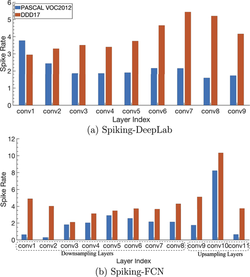
Since MAC operations are based on layer-wise spiking rates, we measure the layer-wise spiking rates of Spiking-DeepLab (figure 14(a)) and Spiking-FCN (figure 14(b)) on two benchmarks (i.e., PASCAL VOC2012 and DDD17). Specifically, we calculate the spike rate Rs(l) of each layer l, which can be defined as the total number of spikes at layer l over total time-steps T divided by the number of neurons in layer l:

Figure 14. Spike rate across all layers in (a) Spiking-DeepLab and (b) Spiking-FCN. We calculate the spike rate for both architectures on PASCAL VOC2012 and DDD17.
Download figure:
Standard image High-resolution imageInterestingly, in figure 14(b), we observe high spike rates in the upsampling layers. This is because of skip connections in Spiking-FCN which inject a number of spikes during forward propagation.
More precisely, following the previous works [25, 36, 71], we compute the energy consumption for SNNs by calculating the total number of floating point operations (FLOPs). Also, to compare ANNs and SNNs quantitatively, we calculate the energy based on standard CMOS technology [72] as shown in table 5. Conventional ANNs require one FP addition and one FP multiplication to conduct the same MAC operation [4]. On the other hand, as the computation of SNNs are event-driven with binary spike processing, the MAC operation reduces to just a floating point (FP) addition. For a layer l in ANNs, we can calculate FLOPs as:

Here, k is kernel size, O is output feature map size, and Cin and Cout are input and output channels, respectively. For SNNs, neurons consume energy whenever the neurons are activated. Thus, we multiply the spiking rate Rs(l) (equation (8)) with FLOPs as:

Finally, the total inference energy of ANNs (EANN) and SNNs (ESNN) across all layers can be obtained using the energy values (EMAC, EAC) from table 5.


Table 5. Energy table for 45 nm CMOS process.
| Operation | Energy (pJ) |
|---|---|
| 32 bit FP MULT (EMULT) | 3.7 |
| 32 bit FP ADD (EADD) | 0.9 |
| 32 bit FP MAC (EMAC) | 4.6 (=EMULT + EADD) |
| 32 bit FP AC (EAC) | 0.9 |
We compare the energy efficiency between ANNs and SNNs on two benchmarks in table 6. As expected, SNNs show higher energy-efficiency (i.e., EANN/Emethod) compared to ANNs. Moreover, we observe that SNNs bring more energy-efficiency on the static VOC2012 dataset since it generates less numbers of spikes across all layers (figure 14). Note that, ANNs have the same energy consumption regardless of datasets whereas SNNs have different energy consumption depending on the number of spikes. It is worth mentioning that SNNs can obtain much higher energy-efficiency on neuromorphic hardware platform [7, 8]. Note that the energy-efficiency results can be changed according to the software/hardware environment. For example, one can use the fuse multiply-add (FMA) operation where the floating-point multiplication and add operations are computed together, which can lead to lower energy consumption for ANNs.
6. Conclusion
In this paper, for the first time, we perform a comprehensive study on the feasibility of training SNNs on the semantic segmentation task. We construct two representative spiking segmentation networks, i.e., Spiking-DeepLab and Spiking-FCN. We show ANN-SNN conversion requires a large number of time-steps (more than one thousand) and shows inferior performance due to the complexity of the segmentation task. This is an important observation since most state-of-the-art SNN training techniques for image recognition are based on ANN-SNN conversion. Instead, we leverage approximated gradient-based training with a temporal batch normalization technique (i.e., BNTT), resulting in reasonable segmentation results with a small number of time-steps. We experimentally evaluate the performance, robustness, and estimated energy on two different semantic segmentation scenarios: the static PASCAL VOC2012 dataset and the DDD17 dataset consisting of event stream spikes. The proposed segmentation architectures can bring a more than 2× energy efficiency on the static image dataset. As future work, we plan to develop an advanced spike-based learning algorithm to fill the performance gap between ANNs and SNNs on semantic segmentation task. Specifically, we will explore how the exact gradient backpropagation calculation [73] improves the performance of event-based segmentation. Furthermore, form the application perspective, semantic segmentation is one of the important applications for unmanned aerial vehicle (UAV) [74, 75] where the primary objective is to understand the layout of the ecosystem. As spiking segmentation brings significant energy-efficiency with proper hardware selection, we hope our research will provide a better intelligent system solution for resource-constrained UAVs.
Acknowledgment
This work was supported in part by C-BRIC, a JUMP center sponsored by DARPA and SRC, Google Research Scholar Award, the National Science Foundation (Grant#1947826), TII (Abu Dhabi) and the DARPA AI Exploration (AIE) program.
Data availability statement
No new data were created or analysed in this study.
