Abstract
The lateral line is a mechanosensory organ found in fish and amphibians that allows them to sense and act on their near-field hydrodynamic environment. We present a 2D-sensitive artificial lateral line (ALL) comprising eight all-optical flow sensors, which we use to measure hydrodynamic velocity profiles along the sensor array in response to a moving object in its vicinity. We then use the measured velocity profiles to reconstruct the object's location, via two types of neural networks: feed-forward and recurrent. Several implementations of feed-forward neural networks for ALL source localisation exist, while recurrent neural networks may be more appropriate for this task. The performance of a recurrent neural network (the long short-term memory, LSTM) is compared to that of a feed-forward neural network (the online-sequential extreme learning machine, OS-ELM) via localizing a 6 cm sphere moving at 13 cm s−1. Results show that, in a 62 cm  9.5 cm area of interest, the LSTM outperforms the OS-ELM with an average localisation error of 0.72 cm compared to 4.27 cm, respectively. Furthermore, the recurrent network is relatively less affected by noise, indicating that recurrent connections can be beneficial for hydrodynamic object localisation.
Original content from this work may be used under the terms of the Creative Commons Attribution 3.0 licence. Any further distribution of this work must maintain attribution to the author(s) and the title of the work, journal citation and DOI.
1. Introduction
The lateral line is a near-field mechanosensory organ found in fish and aquatic amphibians. By measuring water displacement, these animals can detect objects in their vicinity without having to rely on vision or sound (Dijkgraaf 1963). This allows them to perceive predators, peers and prey, even in murky or dark waters. This ability can be referred to as hydrodynamic imaging (Coombs and van Netten 2005, Yang et al 2006) and can be discerned into two modes: active and passive.
In active hydrodynamic imaging, a fish generates a small flow field around themselves through movement. By detecting and measuring distortions in this self-generated flow field, they can detect stationary obstacles. Possible use cases include safe AUV navigation and obstacle avoidance (Kruusmaa et al 2014, Vollmayr et al 2014). In contrast, passive hydrodynamic imaging relies on an external flow field or turbulences. These are generated by other objects that either move or are placed upstream in free stream flow, e.g. Chambers et al (2014) and Zheng et al (2017). This type of sensing could have applications in harbour security or tracking marine life without relying on an active beacon or vision in dark or murky environments.
Most biomimetic implementations of the lateral line, coined artificial lateral lines (ALLs), adhere to passive sensing (Liu et al 2016, Jiang et al 2019); usually, an array of pressure or fluid flow sensors sample the hydrodynamic environment at discrete points which concatenate to spatio-temporal velocity profiles (Franosch et al 2005, Ćurić-Blake and van Netten 2006).
To determine the performance of the ALL and signal processing pipeline, the combined system is usually bench marked via localising a vibrating (dipole), or a moving object, or in one case a moving dipole (Abdulsadda and Tan 2013b).
Several signal processing methods have been put forth to use measured velocity profiles to recover the relative location of the object; thereby partly solving the inverse problem (Abdulsadda and Tan 2013a). These methods include Capon's beamforming (Nguyen et al 2008, Dagamseh et al 2011) and template matching (Ćurić-Blake and van Netten 2006, Pandya et al 2006).
Since the relation between a source location and the resulting sensor signals is quite complex, Abdulsadda and Tan (2011) and Wolf and van Netten (2019) opted to use artificial feed-forward neural networks to perform this source localisation task. The resulting systems were able to accurately detect the location of an object within a region of interest near the sensor array. In a comparative study (Boulogne et al 2017), a recurrent neural network type (ESN) was shown to outperform feedforward neural networks in noisy conditions. This is likely due to the temporal correlation between subsequent object locations and resulting velocity profiles, i.e. temporal context.
In this research, we demonstrate passive hydrodynamic imaging, i.e. localizing a moving object in the vicinity of an artificial lateral line. We compare the performance of two neural network types, feed-forward and recurrent. We hypothesize that recurrent connections may help in localising moving objects, since these networks can inherently make use of temporal context.
2. Background
In this section, we discuss the biological lateral line and our biomimetic implementation, as well as the neural network architectures that support our experiments.
2.1. Lateral line sensing
The lateral line allows fish to perceive a plethora of hydrodynamic phenomena, ranging from movements as small as the water disturbance generated by plankton, to movements as large as river streams (Coombs and van Netten 2005). This phenomenon has been called 'touch at a distance' (Dijkgraaf 1963), and has been associated with behaviours such as schooling, prey detection, rheotaxis, courtship, and station holding (Sutterlin and Waddy 1975, Partridge and Pitcher 1980, Hoekstra and Janssen 1985, Satou et al 1994, Montgomery et al 1997, Coombs and van Netten 2005). Since lateral line perception does not rely on light or sound, it is still effective in environments where these are absent, such as in low-light (e.g. in a dark cave or in blind species) or low-visibility (e.g. murky waters) environments. Fish are capable of detecting sources up to a distance of roughly one fish's body length (Kalmijn 1988, Coombs and Conley 1997, Ćurić-Blake and van Netten 2006).
Lateral lines are comprised of distributed sensors called neuromasts. Two types of neuromasts exist: superficial neuromasts and canal neuromasts. Superficial neuromasts are found on the skin surface all over the fish body, and their number present in one individual ranges from very few up to thousands, depending on the species (Coombs et al 1988). Canal neuromasts are found in fluid-filled canals under the outer skin. The canals themselves can usually be found along the trunk or near the head.
2.2. Sensor array and operation
Many different types of ALL sensors exist, although fluid flow is generally measured through deflection of a cantilever structure (Liu et al 2016). These sensors range from Microelectromechanical systems (MEMS) e.g. Asadnia et al (2016) and ionic polymer-metal composites (IMPC) (Abdulsadda and Tan 2013b) to optical guides (Herzog et al 2015) and, recently, all-optical 2D-sensitive deflection sensors (Wolf et al 2018).
The current all-optical sensor also senses fluid flow via a cantilever deflection. Each sensor contains four optical fibres with fibre Bragg grating (FBG) strain sensing elements. These FBGs reflect a specific wavelength of light, depending on periodic variations in the fibre core. When an individual fibre is strained, the periodic variation stretches or contracts, resulting in a measurable wavelength shift (Flockhart et al 2003). The fluid forces acting on the sensor are thus encoded in the sensor deflection, which can be measured as a linear function of change in reflected wavelength peaks (Wolf et al 2018).
2.3. Neural networks for localization
We discern between two different types of artificial neural networks: feed-forward networks and recurrent networks. The main difference between the two types of networks is the direction of the information flow.
In feed-forward networks, the input strictly moves forward, sequentially going through all layers until it reaches the output layer, which predicts the location of the source.
Conversely, recurrent neural networks have connections which allow the information to not only strictly go forward, but also allow connecting to the same layer, or even to a previous layer. Thanks to these recurrent connections, these networks can take history of the input into account, and are therefore often used when processing temporal data, such as time series.
2.3.1. State of the art
Artificial neural networks, such as the multilayer perceptron (MLP) used by Abdulsadda and Tan (2011) for locating a dipole source, are capable of learning complex, large, non-linear mappings from high-dimensional data sets.
Using simulated data, Boulogne et al (2017) compared the performance of an MLP, an echo state network (ESN) and the extreme learning machine (ELM) (Huang et al 2004) on localizing a moving source under different levels of signal-to-noise ratio. While the ELM outperformed the other algorithms in low noise conditions, the added complexity of the MLP and the recurrency of the ESN allowed these networks to take past velocity profiles into account, which may have caused this type of network to perform better with higher noise levels. This indicates that, under more noisy conditions (such as when using measured data), recurrent networks may be more suitable compared to feed-forward networks.
Specific to the all-optical sensors used in the current study (figure 1), only the ELM architecture has been applied. In Wolf and van Netten (2019), data from an ALL consisting of four sensors was processed by an ELM with 1500 hidden units. The ELM used a time window of 481 ms as the input, which was down sampled to 27 Hz. The combined system was able to predict the location of a 6 cm diameter sphere moving at 7 cm s−1 with an average error of 3.3 cm in an area of  cm.
cm.
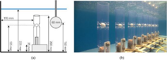
Figure 1. Schematic side view (a) and picture (b) of the 2D-sensitive artificial lateral line (sensor array) situated in the water tank. Eight sensors are placed equidistantly on a 45 cm guiding rail, with perforated protective tubing.
Download figure:
Standard image High-resolution image2.3.2. ELM
For our feed-forward neural network architecture, we make use of a variant of the efficient single layer ELM network. This type of neural network has a single tuneable hyper parameter, the size of the hidden layer, which allows for fast optimization while preventing over fitting. The ELM's input-to-hidden weights  are randomized and fixed (figure 2(a)). This provides a hidden representation
  and leaves only the hidden-to-output weights
  to be learned (Huang et al 2006):

where  denotes the desired (teacher) outputs.
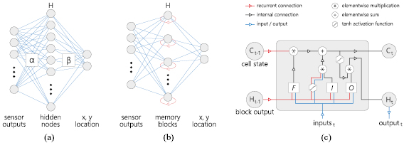
Figure 2. Overview of both neural network structures. (a) OS-ELM network. (b) LSTM network. (c) LSTM memory block. Subfigures (a) and (b) show how the sensor output is propagated to the hidden layer via a set of input weights  . For the OS-ELM, each hidden node sums their input to a hidden value; all hidden values combine to vector H. For the LSTM (b), recurrent connections (red) make H dependent on time. Subfigure (c) further describes the inner mechanics of the memory block. The three gates (F, I, O) receive the past block output and current block inputs. Via multiple operations, the cell state is updated and produces an output.
Download figure:
Standard image High-resolution imageUsing the Moore–Penrose generalized inverse  , the network is able to find optimal weights in a single learning step. An added benefit to the Moore–Penrose generalized inverse is that it produces the smallest norm solution, which also aids avoiding over fitting. This smallest norm, similar to L2-regularization (Goodfellow et al 2016), penalizes large weights and thus penalizes (over-)dependence on single input nodes.
2.3.3. OS-ELM
One consequence of the single learning step, calculating the pseudo-inverse, is that this step becomes computationally intensive with larger data sets. Eventually, it is no longer computationally viable to perform the pseudo-inverse in one step due to hardware, i.e. working memory, constraints. The online sequential ELM (OS-ELM), which functions similarly to the ELM, can deal with larger data sets by implementing a sequential version of the least squares solution algorithm for the inverse operation.
Liang et al (2006) employ a sequential implementation by first calculating output weights based on an initial, sufficiently large, input batch. This initial batch produces a hidden activation or representation  ; consequently, its optimal output weights are calculated using the left pseudo-inverse via:

This produces an initial weights estimate  , optimized for this initial subset. Subsequently, the network is given new input samples in small batches, and the output weight vector is updated based on the discrepancy between the target values of the next subset
  and the estimate based on the previously found weights
  :
:
This second step repeats until all training samples have been processed. In the special case where the initial batch size equals the number of training examples, the OS-ELM implements the original ELM (Liang et al 2006).
2.3.4. LSTM
The long short-term memory (LSTM) network is a recurrent neural network (RNN) capable of learning long-term dependencies. Invented by Hochreiter and Schmidhuber (1997), the LSTM has changed very little since its conception in Hochreiter and Schmidhuber (1997).
Recurrent neural networks are networks in which nodes may have a connection to themselves. This recurrent connection allows them to take earlier inputs into account, giving these networks a temporal dimension. RNNs can therefore detect relations between events which are separated in time (Pascanu et al 2013).
LSTM networks can learn dependencies between samples with a time lag of over 1000 samples (Hochreiter and Schmidhuber 1997). This property has made LSTM networks a popular choice for problems in which long-term memory is needed, such as protein structure prediction (Sønderby et al 2015) and speech recognition (Graves et al 2013).
LSTM networks consist of complex nodes called memory blocks, see figures 2(a) and (c). Each memory block contains a memory cell, whose state is affected by three gates: forget, input, and output. These gates roughly correspond to resetting, writing, and reading operations on this memory cell (Graves 2012).
During the training phase of the network, the gates within the LSTM block are optimized via back propagating the prediction error through time. The steps for updating the input, recurrent, and bias weights as well as the update steps of each type of gate are omitted here and thoroughly described for several variations of the LSTM by Greff et al (2017).
3. Methods
Here, we first describe the setup including the stimulus and sensor array. Then, we discuss the preprocessing steps and how we determine optimal parameters for the neural network implementations and preprocessing methods.
3.1. Setup
Data is gathered in a 1200  800
800  260 mm (w
  l
l  h) water tank. A sphere with a diameter of 6 cm is moved horizontally in this tank by an adapted XY plotter (Makeblock) at a velocity of 13 cm s−1 to create hydrodynamic stimuli. The plotter is controlled with an Arduino-compatible mainboard, which reports its location on set intervals.
The sensor array consists of eight sensors with an inter-sensor distance of 64 mm. One of the eight sensors malfunctioned (see figure 3(a)), and its data is therefore excluded from further analysis, functionally making it a seven-sensor ALL.
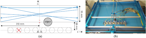
Figure 3. Top view depiction of the setup. Subfigure (a) schematically shows the area of interest, the object, motion paths, and the sensor array. The red cross indicates the excluded sensor. Blue arrows show examples of individual runs. The two red dashes on the y -axis indicate the two distances for the second type of experiments (see section 3.4). Subfigure (b) shows the 2D plotter (blue aluminium beams) with respect to the sensor array. The horizontal blank aluminium bar above the ALL additionally protects the sensors from impact with the object.
Download figure:
Standard image High-resolution imageEach sensor is protected by a perforated 32 mm plastic tube (figure 1) as a failsafe to avoid impacts with the object. The perforation pattern is chosen to be uniform with a ring of eight equidistant 9 mm diameter holes, sandwiched between two rings of eight equidistant 3 mm holes. This allows the bulk of the flow field to enact the sensor, while still providing structural integrity for protection. These perforated tubes may slightly affect the sensor sensitivity (Wolf et al 2018) and introduce a dampening effect; lowering the resonance peak magnitude and frequency, and reducing overall sensitivity.
The measured sensor deflections are obtained via an optical sensing interrogator (Micron Optics si255, Atlanta, USA) at a sampling frequency of 250 Hz. Each sensor is calibrated via a calibration procedure described by Wolf et al (2018). Given that the sensors were calibrated for fluid flow speed outside of their protective tubes, we opt to use the measured deflections as inputs for the neural networks. The expected measured velocity profiles are low frequency (<1 Hz) stimuli, we may therefore assume that the relation between the deflections and fluid velocity is close to linear (Wolf et al 2018).
Both the XY plotter mainbord and the optical sensing interrogator are controlled via a Matlab R2016a script. This allows synchronizing the sensor data with the stimulus location, providing accurate teacher labels for the neural networks.
3.2. Data generation
Object movement is constrained to the (2D) xy-plane; its depth is kept constant during all experiments. The sphere is moved along 256 unique linear paths in a region of interest in front of the array, see figure 3(b). For each path, the sphere is moved back and forth 6 times between the left and right bound, creating a total of 3072 runs.
In addition to the recorded sensor signal, the plotter also provides timestamps for movement initiation, ramp-up, ramp-down, and movement end. These timestamps are used to synchronize and extract the parts of the signal where the velocity is constant; i.e. in between ramp-up and ramp-down. We combine the timestamps with the coordinates given to the plotter to automatically generate location labels for these segments with a constant velocity.
After each plotter movement, the plotter pauses for 20 s in order to minimize the effect of the previous movement on the hydrodynamic situation during subsequent movements.
3.2.1. Preprocessing
For preprocessing, we centre the sensor x- and y -deflections around zero by subtracting their median from the signal. We also investigate the effect of down sampling the signal, which can greatly decrease training time and serves as an additional form of noise reduction. Furthermore, it scales down the temporal dimension, making temporal correlation less distant and easier to learn.
Our parameter sweep for preprocessing includes three different down sampling ratios:  ,
,  , and
, and  .
.
The down sampled data set is subsequently normalized before feeding it to the neural networks. We test the performance using the original data and four variants of normalization techniques, all of which are applied on a per-recording basis:
- 1.none; no further normalization was applied.
- 2.normalize per sensor; for each sensor, scale its time-series so that its maximum amplitude is 1.
- 3.normalize per time step; for each time step, linearly scale the values of all sensors such that the sensor with the largest amplitude has value 1.
- 4.z-score per sensor; for each sensor, transform its time-series to its z-score, giving it mean
 and standard deviation .
 - 5.z-score per time step; for each time step, transform all sensor values with the z-score.


3.3. Neural network optimization
In order to determine the optimal network hyperparameters and preprocessing methods, we perform a parameter sweep for both. We first determine a baseline parameter set which gives a reasonable performance, through trial and error. Then, optimal values for all parameters were found by modifying one variable at a time while keeping others constant, which identifies the effect of that single variable on the performance of the complete pipeline. No grid-wise search is performed due to the excessive time it would take to test each combination.
We further limit the preprocessing parameter sweep to exclude effective time windows that exceed one second, for which we have several reasons. First, longer time windows effectively reduce the amount of training examples, making it harder for generalization to occur. Secondly, longer window sizes may include past data that contains less information and might also be irrelevant for the current location, making it harder to learn temporal patterns from the data. Finally, for time-sensitive tasks, having a smaller window enables a faster response from the neural networks.
3.3.1. LSTM
The LSTM network was implemented in Python using Keras (Chollet et al 2015), a deep learning framework running on top of Tensorflow (Abadi et al 2015). Our LSTM implementation used the Adagrad optimizer with a clipnorm of 1 (Goodfellow et al 2016), which limits calculated gradients such that they cannot exceed a maximum norm of 1, which helps in combatting overfitting.
Data is fed to the LSTM network in batches of windows. Each complete motion in the data set is split up into windows; the default size of the windows is 30 samples, but this value is varied during the parameter sweep. The default window thus has a size of  , for the x- and y - deflections of each of the 7 functioning sensors. Each window is accompanied by a single teacher label corresponding to the ground truth location of the source at the end of that window, creating a many-to-one mapping.
During the parameter sweep, we evaluate the LSTM performance through k-fold cross-validation, with k = 5; this results in a train/test/validation split of 80/10/10%. The order of the 3072 recorded motions is shuffled and each complete motion is assigned to one of the sets.
Based on the parameter sweep (table 1), the optimal LSTM network architecture has 100 hidden nodes, a learning rate ( ) of 0.05, a learning rate decay of
  , no dropout, and uses the hyperbolic tangent activation function (act. fun.). The signal processing pipeline for the LSTM is described by a window size (win sz.) of 15 samples, a stride of 2, a down sampling rate (ds. rate) of 16 (giving the a sampling frequency of 15.625 Hz) and uses, z-score per sensor normalization (norm.).
Table 1. Parameter sweep for the LSTM and signal processing. Indicated here are the default parameters and the variation options for each parameter. From these options, the optimal choices are highlighted in bold.
| Parameter | Default | Options |
|---|---|---|
| Nodes | 50 | 10, 20, 50, 100, 200 |
 |
0.05 | 0.1, 0.05,  , ,  , ,  |
| Decay |  |
0,  , ,  , ,  , ,  |
| Dropout | 0.20 | 0, 0.1, 0.2, 0.35, 0.5 |
| Act. fun. | ReLU | ReLU, sigmoid, tanh |
| win sz. | 30 | 1, 2, 4, 8, 15, 30 |
| Stride | 1 | 1, 2, 4, 8, 15, 30 |
| ds. rate | 8 | 4, 8, 16 |
| Norm. | 4 (z-score) | 1, 2, 3, 4, 5 |
3.3.2. OS-ELM
For the OS-ELM, we similarly divide complete motions from the data set into separate windows, but we also flatten this window to a 1D vector. For the initial training phase, we create a batch of  windows, where N is the number of hidden units. For the sequential training steps, the batch size was set to 64 windows.
Since there is no validation set needed for the OS-ELM training phase, we apply an 80/20% train/test split. Again, with five-fold cross validation, we shuffled the order of the data set and assigned each fold to their respective train or test set.
Table 2 shows the results for the OS-ELM parameter sweep. Based on the parameter sweep, our final ELM network architecture had 30 000 hidden nodes, and uses the ReLU() activation function. The processing pipeline includes a window size of 15 samples, a stride of 1, a down sampling factor of 16 (giving a sampling frequency of 15.625 Hz), and uses z-score normalization.
Table 2. Parameter sweep for the OS-ELM and and signal processing. Indicated here are the default parameters and the variation options for each parameter. From these options, the optimal choices are highlighted in bold.
| Parameter | Default | Options |
|---|---|---|
| Nodes | 5000 | {1, 2, 5, 10, 20, 30}  |
| act. fun. | sigmoid | ReLU, sigmoid, tanh |
| win sz. | 30 | 1, 2, 4, 8, 15, 30 |
| Stride | 1 | 1, 2, 4, 8, 15, 30 |
| ds. rate | 8 | 4, 8, 16 |
| Norm. | 4 (z-score) | 1, 2, 3, 4, 5 |
The constant speed section of each motion lasts between 4.3 s for horizontal and 4.5 s for diagonal motion. This results in a data set of  input examples for the OS-ELM. For the LSTM framework, given the stride of 2 rather than 1, the data set is roughly half that size.
Although the number of hidden nodes for the OS-ELM may seem high, the number of input examples (windows) is roughly 7 times higher. This makes it unlikely for overfitting to occur.
3.4. Influence of noise
We create a separate data set in order to systematically determine the influence of noise. In particular, we are interested in the localization robustness of the two types of neural networks with respect to different noise levels. This data set consists of 60 repetitions of both backwards and forward motion along two unique paths parallel to the array, at 6.15 cm and 8.15 cm distance, respectively, producing 240 recorded motions. These distances are indicated via red dashes in figure 3(a).
For augmenting this data set, we employ a controlled method of adding noise to our data; we want to stay as close to the real environment as possible, while still being able to quantify how much noise is added. We therefore first record a large data set without any stimulus or plotter activity, from which we sample noise specific to each sensor. We augment the data set by combining recordings with the following nine noise augmentation amplification levels: {0, 0.1, 0.25, 0.5, 1, 1.5, 2, 3, 4}, producing a final augmented set of 2160 motions. This range is selected on a pseudo-logarithmic scale to allow testing a large range of noise levels.
We keep the previously determined optimal hyper parameters for both type of neural networks and thus do not re-optimize for this augmented data set. For determining the performance of each network, we employ five-fold proportional stratified sampling; each of the five folds has an equal amount of randomly picked complete motions from each of the nine augmented sets. The training data is shuffled before using these folds for training the networks.
4. Results
4.1. Localisation performance
In the first series of experiments, we compared the performance of a feed-forward neural network (OS-ELM) to the performance of a recurrent neural network (LSTM) on the task of localizing a source using measured artificial lateral line (ALL) data.
Both networks were optimized with respect to their hyper parameters and preprocessing methods using five-fold cross validation, as described in the Methods section.
Figure 4 shows an example of a single run, where both networks predict the location of an object moving parallel to the array. This figure shows that the LSTM network output is less erratic and closer to the target path compared to the ELM prediction.
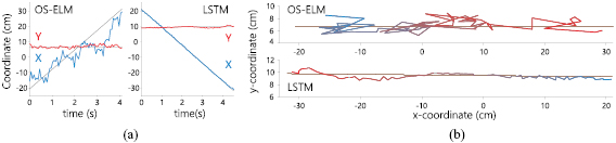
Figure 4. Predicted and true labels for one example run. Subfigure (a) shows the true coordinates over time (black lines) as well as the prediction of the OS-ELM and LSTM for the x-coordinate (blue) and y -coordinate (red). Subfigure (b) shows the true path of motion (black lines) and the reconstructed path (blue to red over time) for both networks.
Download figure:
Standard image High-resolution imageWhen we combine and interpolate between all locations in the region of interest, we can show a spatial mapping of the localisation error. Figure 5 shows the interpolated error magnitude at each location. From these spatial plots, we observe that the localisation error further away from the array increases for both neural networks.
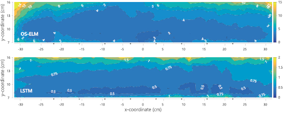
Figure 5. Spatial distribution of localisation errors (cm) for both type of networks. Note that the colour bars are scaled per network, up to 15 cm error for the OS-ELM and only up to 2 cm error for the better performing LSTM. The small dots on the x-axis indicate the x-coordinates of each sensor.
Download figure:
Standard image High-resolution imageThe actual distribution of localisation errors, regardless of relative location, is shown in figure 6(a). Here, we binned the localisation error for both types of networks, with a limit of 15 cm. The average and standard deviation of the localisation errors are  cm and
  cm for the LSTM and OS-ELM, respectively. While the LSTM errors are concentrated around the average, the OS-ELM has a large tail in the distribution (figure 6(a)), with 4.2% of the errors exceeding 15 cm (not shown).
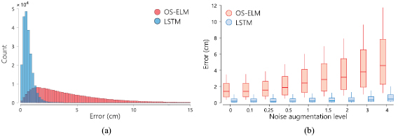
Figure 6. Subfigure (a) shows the error distribution for the first set of experiments, which has a significant different shape for both networks. Subfigure (b) shows the median error (bold line) and confidence intervals for different noise augmentation levels for the second set of experiments. Here, we show 10, 25, 50, 75, and 90% confidence levels.
Download figure:
Standard image High-resolution imageThese results show that the LSTM network significantly outperforms the OS-ELM network on this 2D source localisation task using measured velocity profiles from a 2D-sensitive array.
4.2. Noise robustness
To further determine the suitability of both neural networks for other circumstances or other types of artificial lateral lines, we also investigated the effect of noise with respect to localisation.
In our performance analysis, we differentiate between noise augmentation levels within the test set. Figure 6(b) and table 3 both provide an insight in the effect of added noise to the overall performance. As the noise level increases, so do the LSTM and OS-ELM network's average localization errors, although the LSTM seems relatively less affected by higher noise levels.
Table 3. Error per noise level for LSTM and OS-ELM networks after stratified five-fold cross-validation. Shown here are the mean Euclidean error and standard deviation. Finally, the average error over all noise levels is shown.
| Noise level | LSTM error ( cm) cm) |
OS-ELM error ( cm) cm) |
|---|---|---|
| 0.00 |  |
 |
| 0.10 |  |
 |
| 0.25 |  |
 |
| 0.50 |  |
 |
| 1.00 |  |
 |
| 1.50 |  |
 |
| 2.00 |  |
 |
| 3.00 |  |
 |
| 4.00 |  |
 |
| Average |  |
 |
Figure 6(b) shows box plots of OS-ELM and LSTM performance, separated per noise level. For all noise levels considered, the median LSTM error is significantly lower than the OS-ELM error.
Table 3 shows the overall and per-noise-level error for both networks. On the lowest noise level (no noise), the LSTM achieved an average error of 0.55 cm, whereas the ELM had an average error of 1.75 cm. For the highest noise level (4 ), these errors increase to 1.10 cm and 5.64 cm for the LSTM and ELM networks, respectively. Again, the error distribution of the OS-ELM shows a long tail towards higher errors, making it less reliable than the LSTM in this comparison.
5. Discussion
The aim of our research was to determine how well recurrent neural networks performed compared to feed-forward neural networks, which are the current state of the art, on the task of processing measured artificial lateral line data.
Based on the results from our first series of experiments, we can safely conclude that the recurrent neural network (LSTM) is able to accurately estimate moving underwater source locations. Furthermore, the LSTM network outperformed the OS-ELM network, with an average localization error of 0.72 cm for the LSTM compared to average error of 4.27 cm for the OS-ELM. While this result may not generalize to all feed-forward and recurrent networks, it does indicate that recurrent networks may be more suited to processing ALL data than some feed-forward networks.
Overall, the spatial mapping of localisation errors indicate that objects moving at distances further away from the array are harder to localize. This is in agreement with other research and with theory; i.e. the signal to noise ratio of measured and expected velocity profiles negatively correlate with distance.
The omitted malfunctioning sensor does not significantly affect the (local) spatial localisation errors as indicated in figure 5. On average, the left half of the region of interest (with the omitted sensor) has slightly higher errors. It is unclear why this effect is limited, although it might be a result of the unbiased optimization nature of neural networks; all locations are treated with equal importance. In the case of object detection or obstacle avoidance, nearby locations may be considered more relevant. A more advanced localisation algorithm may consider a weighted optimization error metric, depending on the distance of a target location to each (functioning) sensor in the array, as an approximation to Fisher information or the Cramer–Rao bound (Abdulsadda and Tan 2013a).
The signal-to-noise ratio of the measured velocity profile of an object highly depends on its size, speed, and distance with respect to the array. The specific sensor array sensitivity also influences this ratio. The second, augmented data set with varying noise levels allowed us to assess the performance of both network types under influence of sensor noise, independent of object distance. By changing and varying the input noise, we can effectively emulate different (lower) sensor array sensitivities, which makes the findings more applicable to situations with a lower signal to noise ratio. The average localization errors are 0.69 cm and 3.16 cm for the LSTM and OS-ELM networks, respectively. Furthermore, while both networks decrease in performance with higher noise levels, the LSTM is clearly less affected, suggesting that recurrent connections may help in alleviating the effects of random, uncorrelated input noise.
Our current sensor array of 45 cm with 7 functional 2D-sensitive all-optical sensors in combination with our LSTM implementation leads to an average localisation error of 0.72 cm in a region of interest of  cm. This result cannot be easily directly compared to the state of the art, because other works use other type of sensors and other relative dimensions for their sensor array and region of interest (Jiang et al 2019). Furthermore, most studies only consider stationary vibrating (see Abdulsadda and Tan (2011)) or moving vibrating objects (Abdulsadda and Tan 2013b); the stimulation frequency can be used to filter the signal and thus produces higher signal-to-noise data than possible for non-vibrating moving objects.
In one similar study, Wolf and van Netten (2019) show an 3.3 cm localisation error for a moving sphere with a four-sensor array of 12 cm in an area of  cm using an ELM. The maximal distance of the current study is similar, while both the region of interest and sensor array array are considerably wider. We therefore conclude that the OS-ELM performance is on par while the LSTM implementation outperforms the state of the art for unidirectionally moving objects with constant velocity.
There are two main considerations for future work and expansions to our experiments. First, although our stimulus is more complex than the standard dipole bench mark, the motion was still restricted at one depth-level and in a straight line with constant speed. This type of motion naturally favours taking longer time windows and using memory (i.e. recurrent connections), since the path of the object is predictable.
For future demonstrations of versatile artificial lateral line hydrodynamic imaging, one could consider more complex object propulsion and object shapes. These bench mark stimuli are limited in the sense that they do not emulate fish motion (Zheng et al 2017) or aquatic propulsion, but rather they provide a controlled, fair comparison method. By using a moving, rather than vibrating, source, we increased the complexity of the hydrodynamic environment by allowing wakes and vortices to be measured by the sensor array. This is however no substitution for detecting an object in freestream flow or in a hydrodynamic environment with multiple objects or alternative flow sources. Future research could explore localizing self-propelling objects using a stationary artificial lateral line.
Secondly, while the LSTM is quite an advanced network, the OS-ELM is limited in its complexity. Future research could compare more complex feed-forward neural networks or simpler recurrent neural networks, to further investigate the effect of recurrence versus network complexity. In one simulation study (Boulogne et al 2017), the ELM and echo state network (ESN) are compared where they have similar levels of performance. In this regard, the ESN is an interesting comparison candidate: it has recurrent connections although the network structure closely resembles the ELM.
6. Conclusion
In conclusion, a system with recurrent neural networks is capable of hydrodynamic imaging; i.e. localizing a moving underwater source in a 2D plane based on measurements with a 2D-sensitive artificial lateral line of all-optical sensors. This type of passive object sensing does not rely on vision or an active beacon and can therefore work in dark or murky environments. It may therefore, despite its limited range, be favoured over traditional detection technologies when considering ecology or covert sensing.
The recurrent network (LSTM) significantly outperforms the feed-forward network (OS-ELM) for localizing a moving object in quiescent water. This may be due to the temporal correlation between subsequent object locations and the resulting subsequent measured velocity patterns. In addition, the recurrent network is relatively less affected by sensing noise, and performs more consistently throughout the area of interest. This indicates that recurrent neural networks may be especially suited for hydrodynamic imaging.
Acknowledgments
This research has been supported by the Lakhsmi project that has received funding from the European Union's Horizon 2020 research and innovation program under Grant agreement No. 635568.