Remove ads
In signal processing and statistics, a window function (also known as an apodization function or tapering function[1]) is a mathematical function that is zero-valued outside of some chosen interval. Typically, window functions are symmetric around the middle of the interval, approach a maximum in the middle, and taper away from the middle. Mathematically, when another function or waveform/data-sequence is "multiplied" by a window function, the product is also zero-valued outside the interval: all that is left is the part where they overlap, the "view through the window". Equivalently, and in actual practice, the segment of data within the window is first isolated, and then only that data is multiplied by the window function values. Thus, tapering, not segmentation, is the main purpose of window functions.
The reasons for examining segments of a longer function include detection of transient events and time-averaging of frequency spectra. The duration of the segments is determined in each application by requirements like time and frequency resolution. But that method also changes the frequency content of the signal by an effect called spectral leakage. Window functions allow us to distribute the leakage spectrally in different ways, according to the needs of the particular application. There are many choices detailed in this article, but many of the differences are so subtle as to be insignificant in practice.
In typical applications, the window functions used are non-negative, smooth, "bell-shaped" curves.[2] Rectangle, triangle, and other functions can also be used. A more general definition of window functions does not require them to be identically zero outside an interval, as long as the product of the window multiplied by its argument is square integrable, and, more specifically, that the function goes sufficiently rapidly toward zero.[3]
Remove ads
Window functions are used in spectral analysis/modification/resynthesis,[4] the design of finite impulse response filters, merging multiscale and multidimensional datasets,[5][6] as well as beamforming and antenna design.

Spectral analysis
The Fourier transform of the function cos(ωt) is zero, except at frequency ±ω. However, many other functions and waveforms do not have convenient closed-form transforms. Alternatively, one might be interested in their spectral content only during a certain time period.
In either case, the Fourier transform (or a similar transform) can be applied on one or more finite intervals of the waveform. In general, the transform is applied to the product of the waveform and a window function. Any window (including rectangular) affects the spectral estimate computed by this method.
Filter design
Windows are sometimes used in the design of digital filters, in particular to convert an "ideal" impulse response of infinite duration, such as a sinc function, to a finite impulse response (FIR) filter design. That is called the window method.[7][8][9]
Statistics and curve fitting
Window functions are sometimes used in the field of statistical analysis to restrict the set of data being analyzed to a range near a given point, with a weighting factor that diminishes the effect of points farther away from the portion of the curve being fit. In the field of Bayesian analysis and curve fitting, this is often referred to as the kernel.
Rectangular window applications
Analysis of transients
When analyzing a transient signal in modal analysis, such as an impulse, a shock response, a sine burst, a chirp burst, or noise burst, where the energy vs time distribution is extremely uneven, the rectangular window may be most appropriate. For instance, when most of the energy is located at the beginning of the recording, a non-rectangular window attenuates most of the energy, degrading the signal-to-noise ratio.[10]
Harmonic analysis
One might wish to measure the harmonic content of a musical note from a particular instrument or the harmonic distortion of an amplifier at a given frequency. Referring again to Figure 2, we can observe that there is no leakage at a discrete set of harmonically-related frequencies sampled by the discrete Fourier transform (DFT). (The spectral nulls are actually zero-crossings, which cannot be shown on a logarithmic scale such as this.) This property is unique to the rectangular window, and it must be appropriately configured for the signal frequency, as described above.
Remove ads
When the length of a data set to be transformed is larger than necessary to provide the desired frequency resolution, a common practice is to subdivide it into smaller sets and window them individually. To mitigate the "loss" at the edges of the window, the individual sets may overlap in time. See Welch method of power spectral analysis and the modified discrete cosine transform.
Two-dimensional windows are commonly used in image processing to reduce unwanted high-frequencies in the image Fourier transform.[11] They can be constructed from one-dimensional windows in either of two forms.[12] The separable form, is trivial to compute. The radial form, , which involves the radius , is isotropic, independent on the orientation of the coordinate axes. Only the Gaussian function is both separable and isotropic.[13] The separable forms of all other window functions have corners that depend on the choice of the coordinate axes. The isotropy/anisotropy of a two-dimensional window function is shared by its two-dimensional Fourier transform. The difference between the separable and radial forms is akin to the result of diffraction from rectangular vs. circular apertures, which can be visualized in terms of the product of two sinc functions vs. an Airy function, respectively.
Remove ads
Conventions:
- is a zero-phase function (symmetrical about ),[14] continuous for where is a positive integer (even or odd).[15]
- The sequence is symmetric, of length
- is DFT-symmetric, of length [A]
- The parameter B displayed on each spectral plot is the function's noise equivalent bandwidth metric, in units of DFT bins.[16]: p.56 eq.(16)
- See spectral leakage §§ Discrete-time signals and Some window metrics and Normalized frequency for understanding the use of "bins" for the x-axis in these plots.
The sparse sampling of a discrete-time Fourier transform (DTFT) such as the DFTs in Fig 2 only reveals the leakage into the DFT bins from a sinusoid whose frequency is also an integer DFT bin. The unseen sidelobes reveal the leakage to expect from sinusoids at other frequencies.[a] Therefore, when choosing a window function, it is usually important to sample the DTFT more densely (as we do throughout this section) and choose a window that suppresses the sidelobes to an acceptable level.
Rectangular window

The rectangular window (sometimes known as the boxcar or uniform or Dirichlet window or misleadingly as "no window" in some programs[18]) is the simplest window, equivalent to replacing all but N consecutive values of a data sequence by zeros, making the waveform suddenly turn on and off:
Other windows are designed to moderate these sudden changes, to reduce scalloping loss and improve dynamic range (described in § Spectral analysis).
The rectangular window is the 1st-order B-spline window as well as the 0th-power power-of-sine window.
The rectangular window provides the minimum mean square error estimate of the Discrete-time Fourier transform, at the cost of other issues discussed.
B-spline windows
B-spline windows can be obtained as k-fold convolutions of the rectangular window. They include the rectangular window itself (k = 1), the § Triangular window (k = 2) and the § Parzen window (k = 4).[19] Alternative definitions sample the appropriate normalized B-spline basis functions instead of convolving discrete-time windows. A kth-order B-spline basis function is a piece-wise polynomial function of degree k − 1 that is obtained by k-fold self-convolution of the rectangular function.
Triangular window
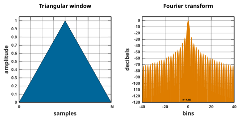
Triangular windows are given by
where L can be N,[20] N + 1,[16][21][22] or N + 2.[23] The first one is also known as Bartlett window or Fejér window. All three definitions converge at large N.
The triangular window is the 2nd-order B-spline window. The L = N form can be seen as the convolution of two N⁄2-width rectangular windows. The Fourier transform of the result is the squared values of the transform of the half-width rectangular window.
Parzen window

Defining L ≜ N + 1, the Parzen window, also known as the de la Vallée Poussin window,[16] is the 4th-order B-spline window given by

Other polynomial windows
Welch window
The Welch window consists of a single parabolic section:
The defining quadratic polynomial reaches a value of zero at the samples just outside the span of the window.
Sine window

The corresponding function is a cosine without the π/2 phase offset. So the sine window[24] is sometimes also called cosine window.[16] As it represents half a cycle of a sinusoidal function, it is also known variably as half-sine window[25] or half-cosine window.[26]
The autocorrelation of a sine window produces a function known as the Bohman window.[27]
Power-of-sine/cosine windows
These window functions have the form:[28]
The rectangular window (α = 0), the sine window (α = 1), and the Hann window (α = 2) are members of this family.
For even-integer values of α these functions can also be expressed in cosine-sum form:
Cosine-sum windows
This family is also known as generalized cosine windows.
| Eq.1 |
In most cases, including the examples below, all coefficients ak ≥ 0. These windows have only 2K + 1 non-zero N-point DFT coefficients.
Hann and Hamming windows
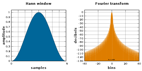

The customary cosine-sum windows for case K = 1 have the form
which is easily (and often) confused with its zero-phase version:
Setting produces a Hann window:
named after Julius von Hann, and sometimes erroneously referred to as Hanning, presumably due to its linguistic and formulaic similarities to the Hamming window. It is also known as raised cosine, because the zero-phase version, is one lobe of an elevated cosine function.
This function is a member of both the cosine-sum and power-of-sine families. Unlike the Hamming window, the end points of the Hann window just touch zero. The resulting side-lobes roll off at about 18 dB per octave.[30]
Setting to approximately 0.54, or more precisely 25/46, produces the Hamming window, proposed by Richard W. Hamming. This choice places a zero crossing at frequency 5π/(N − 1), which cancels the first sidelobe of the Hann window, giving it a height of about one-fifth that of the Hann window.[16][31][32] The Hamming window is often called the Hamming blip when used for pulse shaping.[33][34][35]
Approximation of the coefficients to two decimal places substantially lowers the level of sidelobes,[16] to a nearly equiripple condition.[32] In the equiripple sense, the optimal values for the coefficients are a0 = 0.53836 and a1 = 0.46164.[32][36]
Blackman window
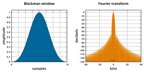
Blackman windows are defined as
By common convention, the unqualified term Blackman window refers to Blackman's "not very serious proposal" of α = 0.16 (a0 = 0.42, a1 = 0.5, a2 = 0.08), which closely approximates the exact Blackman,[37] with a0 = 7938/18608 ≈ 0.42659, a1 = 9240/18608 ≈ 0.49656, and a2 = 1430/18608 ≈ 0.076849.[38] These exact values place zeros at the third and fourth sidelobes,[16] but result in a discontinuity at the edges and a 6 dB/oct fall-off. The truncated coefficients do not null the sidelobes as well, but have an improved 18 dB/oct fall-off.[16][39]
Nuttall window, continuous first derivative

The continuous form of the Nuttall window, and its first derivative are continuous everywhere, like the Hann function. That is, the function goes to 0 at x = ±N/2, unlike the Blackman–Nuttall, Blackman–Harris, and Hamming windows. The Blackman window (α = 0.16) is also continuous with continuous derivative at the edge, but the "exact Blackman window" is not.
Blackman–Nuttall window

Blackman–Harris window

A generalization of the Hamming family, produced by adding more shifted sinc functions, meant to minimize side-lobe levels[40][41]
Flat top window
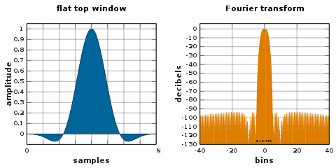
A flat top window is a partially negative-valued window that has minimal scalloping loss in the frequency domain. That property is desirable for the measurement of amplitudes of sinusoidal frequency components.[17][42] However, its broad bandwidth results in high noise bandwidth and wider frequency selection, which depending on the application could be a drawback.
Flat top windows can be designed using low-pass filter design methods,[42] or they may be of the usual cosine-sum variety:
The Matlab variant has these coefficients:
Other variations are available, such as sidelobes that roll off at the cost of higher values near the main lobe.[17]
Rife–Vincent windows
Rife–Vincent windows[43] are customarily scaled for unity average value, instead of unity peak value. The coefficient values below, applied to Eq.1, reflect that custom.
Class I, Order 1 (K = 1): Functionally equivalent to the Hann window.
Class I, Order 2 (K = 2):
Class I is defined by minimizing the high-order sidelobe amplitude. Coefficients for orders up to K=4 are tabulated.[44]
Class II minimizes the main-lobe width for a given maximum side-lobe.
Class III is a compromise for which order K = 2 resembles the § Blackman window.[44][45]
Adjustable windows
Gaussian window
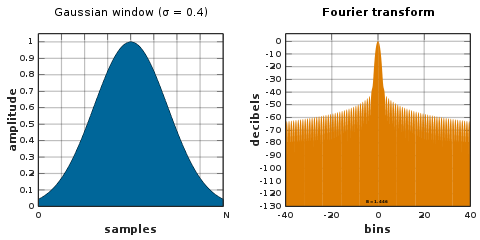
The Fourier transform of a Gaussian is also a Gaussian. Since the support of a Gaussian function extends to infinity, it must either be truncated at the ends of the window, or itself windowed with another zero-ended window.[46]
Since the log of a Gaussian produces a parabola, this can be used for nearly exact quadratic interpolation in frequency estimation.[47][46][48]
The standard deviation of the Gaussian function is σ · N/2 sampling periods.
Confined Gaussian window
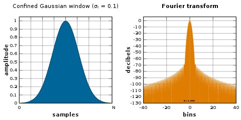
The confined Gaussian window yields the smallest possible root mean square frequency width σω for a given temporal width (N + 1) σt.[49] These windows optimize the RMS time-frequency bandwidth products. They are computed as the minimum eigenvectors of a parameter-dependent matrix. The confined Gaussian window family contains the § Sine window and the § Gaussian window in the limiting cases of large and small σt, respectively.

Approximate confined Gaussian window
Defining L ≜ N + 1, a confined Gaussian window of temporal width L × σt is well approximated by:[49]
where is a Gaussian function:
The standard deviation of the approximate window is asymptotically equal (i.e. large values of N) to L × σt for σt < 0.14.[49]
Generalized normal window
A more generalized version of the Gaussian window is the generalized normal window.[50] Retaining the notation from the Gaussian window above, we can represent this window as
for any even . At , this is a Gaussian window and as approaches , this approximates to a rectangular window. The Fourier transform of this window does not exist in a closed form for a general . However, it demonstrates the other benefits of being smooth, adjustable bandwidth. Like the § Tukey window, this window naturally offers a "flat top" to control the amplitude attenuation of a time-series (on which we don't have a control with Gaussian window). In essence, it offers a good (controllable) compromise, in terms of spectral leakage, frequency resolution and amplitude attenuation, between the Gaussian window and the rectangular window. See also [51] for a study on time-frequency representation of this window (or function).
Tukey window

The Tukey window, also known as the cosine-tapered window, can be regarded as a cosine lobe of width Nα/2 (spanning Nα/2 + 1 observations) that is convolved with a rectangular window of width N(1 − α/2).
At α = 0 it becomes rectangular, and at α = 1 it becomes a Hann window.
Planck-taper window

The so-called "Planck-taper" window is a bump function that has been widely used[53] in the theory of partitions of unity in manifolds. It is smooth (a function) everywhere, but is exactly zero outside of a compact region, exactly one over an interval within that region, and varies smoothly and monotonically between those limits. Its use as a window function in signal processing was first suggested in the context of gravitational-wave astronomy, inspired by the Planck distribution.[54] It is defined as a piecewise function:
The amount of tapering is controlled by the parameter ε, with smaller values giving sharper transitions.
DPSS or Slepian window
The DPSS (discrete prolate spheroidal sequence) or Slepian window maximizes the energy concentration in the main lobe,[55] and is used in multitaper spectral analysis, which averages out noise in the spectrum and reduces information loss at the edges of the window.
The main lobe ends at a frequency bin given by the parameter α.[56]
 |
 |
The Kaiser windows below are created by a simple approximation to the DPSS windows:
 |
 |
Kaiser window
The Kaiser, or Kaiser–Bessel, window is a simple approximation of the DPSS window using Bessel functions, discovered by James Kaiser.[57][58]
where is the 0th-order modified Bessel function of the first kind. Variable parameter determines the tradeoff between main lobe width and side lobe levels of the spectral leakage pattern. The main lobe width, in between the nulls, is given by in units of DFT bins,[65] and a typical value of is 3.
Dolph–Chebyshev window

Minimizes the Chebyshev norm of the side-lobes for a given main lobe width.[66]
The zero-phase Dolph–Chebyshev window function is usually defined in terms of its real-valued discrete Fourier transform, :[67]
Tn(x) is the n-th Chebyshev polynomial of the first kind evaluated in x, which can be computed using
and
is the unique positive real solution to , where the parameter α sets the Chebyshev norm of the sidelobes to −20α decibels.[66]
The window function can be calculated from W0(k) by an inverse discrete Fourier transform (DFT):[66]
The lagged version of the window can be obtained by:
which for even values of N must be computed as follows:
which is an inverse DFT of
Variations:
- Due to the equiripple condition, the time-domain window has discontinuities at the edges. An approximation that avoids them, by allowing the equiripples to drop off at the edges, is a Taylor window.
- An alternative to the inverse DFT definition is also available..
Ultraspherical window

The Ultraspherical window was introduced in 1984 by Roy Streit[68] and has application in antenna array design,[69] non-recursive filter design,[68] and spectrum analysis.[70]
Like other adjustable windows, the Ultraspherical window has parameters that can be used to control its Fourier transform main-lobe width and relative side-lobe amplitude. Uncommon to other windows, it has an additional parameter which can be used to set the rate at which side-lobes decrease (or increase) in amplitude.[70][71][72]
The window can be expressed in the time-domain as follows:[70]
where is the Ultraspherical polynomial of degree N, and and control the side-lobe patterns.[70]
Certain specific values of yield other well-known windows: and give the Dolph–Chebyshev and Saramäki windows respectively.[68] See here for illustration of Ultraspherical windows with varied parametrization.
Exponential or Poisson window


The Poisson window, or more generically the exponential window increases exponentially towards the center of the window and decreases exponentially in the second half. Since the exponential function never reaches zero, the values of the window at its limits are non-zero (it can be seen as the multiplication of an exponential function by a rectangular window [73]). It is defined by
where τ is the time constant of the function. The exponential function decays as e ≃ 2.71828 or approximately 8.69 dB per time constant.[74] This means that for a targeted decay of D dB over half of the window length, the time constant τ is given by
Hybrid windows
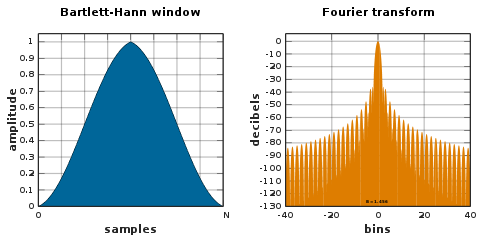
Window functions have also been constructed as multiplicative or additive combinations of other windows.
Bartlett–Hann window
Planck–Bessel window

A § Planck-taper window multiplied by a Kaiser window which is defined in terms of a modified Bessel function. This hybrid window function was introduced to decrease the peak side-lobe level of the Planck-taper window while still exploiting its good asymptotic decay.[75] It has two tunable parameters, ε from the Planck-taper and α from the Kaiser window, so it can be adjusted to fit the requirements of a given signal.
Hann–Poisson window

A Hann window multiplied by a Poisson window. For it has no side-lobes, as its Fourier transform drops off forever away from the main lobe without local minima. It can thus be used in hill climbing algorithms like Newton's method.[76] The Hann–Poisson window is defined by:
where α is a parameter that controls the slope of the exponential.
Other windows

Generalized adaptive polynomial (GAP) window
The GAP window is a family of adjustable window functions that are based on a symmetrical polynomial expansion of order . It is continuous with continuous derivative everywhere. With the appropriate set of expansion coefficients and expansion order, the GAP window can mimic all the known window functions, reproducing accurately their spectral properties.
where is the standard deviation of the sequence.
Additionally, starting with a set of expansion coefficients that mimics a certain known window function, the GAP window can be optimized by minimization procedures to get a new set of coefficients that improve one or more spectral properties, such as the main lobe width, side lobe attenuation, and side lobe falloff rate.[78] Therefore, a GAP window function can be developed with designed spectral properties depending on the specific application.

Lanczos window
- used in Lanczos resampling
- for the Lanczos window, is defined as
- also known as a sinc window, because: is the main lobe of a normalized sinc function
Asymmetric window functions
The form, according to the convention above, is symmetric around . However, there are window functions that are asymmetric, such as the Gamma distribution used in FIR implementations of Gammatone filters. These asymmetries are used to reduce the delay when using large window sizes, or to emphasize the initial transient of a decaying pulse.[citation needed]
Any bounded function with compact support, including asymmetric ones, can be readily used as a window function. Additionally, there are ways to transform symmetric windows into asymmetric windows by transforming the time coordinate, such as with the below formula
where the window weights more highly the earliest samples when 1}">, and conversely weights more highly the latest samples when .[79]
Remove ads
- This formula can be confirmed by simplifying the cosine function at MATLAB tukeywin and substituting r=α and x=n/N.
- Harris 1978 (p 67, eq 38) appears to have two errors: (1) The subtraction operator in the numerator of the cosine function should be addition. (2) The denominator contains a spurious factor of 2. Also, Fig 30 corresponds to α=0.25 using the Wikipedia formula, but to 0.75 using the Harris formula. Fig 32 is similarly mislabeled.
Remove ads
- Harris 1978, p 57, fig 10.
Wikiwand in your browser!
Seamless Wikipedia browsing. On steroids.
Every time you click a link to Wikipedia, Wiktionary or Wikiquote in your browser's search results, it will show the modern Wikiwand interface.
Wikiwand extension is a five stars, simple, with minimum permission required to keep your browsing private, safe and transparent.
Remove ads