Nothing Special   »   [go: up one dir, main page]

You seem to have javascript disabled. Please note that many of the page functionalities won't work as expected without javascript enabled.


Predictive and Learning Control in Engineering Applications

A topical collection in Electronics (ISSN 2079-9292). This collection belongs to the section "Systems & Control Engineering".

Viewed by 52183

Editors


E-Mail Website
Collection Editor
Autonomous Systems and Robotics Lab, Computer Science and System Engineering Department (U2IS), École Nationale Supérieure de Techniques Avancées (ENSTA Paris), Institut Polytechnique de Paris (IP Paris), 828 Boulevard des Maréchaux, 91120 Palaiseau, France
Interests: H∞ control; gain scheduling; control allocation; vehicle dynamics; co-simulation; robust control; model predictive control; optimal control
Special Issues, Collections and Topics in MDPI journals

E-Mail Website
Collection Editor
Autonomous Systems and Robotics Lab, Computer Science and System Engineering Department (U2IS), École Nationale Supérieure de Techniques Avancées (ENSTA Paris), Institut Polytechnique de Paris (IP Paris), 828 Boulevard des Maréchaux, 91120 Palaiseau, France

E-Mail Website
Collection Editor
Department of Cognitive Robotics, Delft University of Technology, 2628 CD Delft, The Netherlands
Interests: vehicle dynamics and control; automated driving; model predictive control; optimal control
Special Issues, Collections and Topics in MDPI journals

Topical Collection Information

Dear Colleagues,

In many control design problems, a model-based approach is chosen. This approach has proven its effectiveness in several engineering applications as long as the dynamics involved are known and analytically describable. Nevertheless, even if the dynamics are uncertain, robust controllers can be designed to ensure the stability of the studied system in spite of the uncertainty. The problem is that classic robust control design suffers from conservatism, which reduces the performance of the controller.

Since the limitation comes from uncertainty, if the dynamics could be known precisely, the problem would be solved. Thanks to learning-based identification, the modeling of the dynamics can be improved. Once the modeling is improved, a predictive control could be applied to achieve an optimal solution.

This Topical Collection focuses on recent advances in the design, validation, and implementation of predictive and learning-based control strategies. This Topical Collection is not limited to a specific application, and all engineering applications are welcome.

Dr. Moad Kissai
Prof. Dr. Bruno Monsuez
Dr. Barys Shyrokau
Collection Editors

Manuscript Submission Information

Manuscripts should be submitted online at www.mdpi.com by registering and logging in to this website. Once you are registered, click here to go to the submission form. Manuscripts can be submitted until the deadline. All submissions that pass pre-check are peer-reviewed. Accepted papers will be published continuously in the journal (as soon as accepted) and will be listed together on the collection website. Research articles, review articles as well as short communications are invited. For planned papers, a title and short abstract (about 100 words) can be sent to the Editorial Office for announcement on this website.

Submitted manuscripts should not have been published previously, nor be under consideration for publication elsewhere (except conference proceedings papers). All manuscripts are thoroughly refereed through a single-blind peer-review process. A guide for authors and other relevant information for submission of manuscripts is available on the Instructions for Authors page. Electronics is an international peer-reviewed open access semimonthly journal published by MDPI.

Please visit the Instructions for Authors page before submitting a manuscript. The Article Processing Charge (APC) for publication in this open access journal is 2400 CHF (Swiss Francs). Submitted papers should be well formatted and use good English. Authors may use MDPI's English editing service prior to publication or during author revisions.

Keywords

  • predictive control
  • learning-based identification
  • learning-based control
  • optimal control
  • adaptive control

Published Papers (27 papers)

2024

Jump to: 2023, 2022, 2021

27 pages, 2352 KiB  
Article
LEVIOSA: Natural Language-Based Uncrewed Aerial Vehicle Trajectory Generation
by Godwyll Aikins, Mawaba Pascal Dao, Koboyo Josias Moukpe, Thomas C. Eskridge and Kim-Doang Nguyen
Electronics 2024, 13(22), 4508; https://doi.org/10.3390/electronics13224508 (registering DOI) - 17 Nov 2024
Viewed by 124
Abstract
This paper presents LEVIOSA, a novel framework for text- and speech-based uncrewed aerial vehicle (UAV) trajectory generation. By leveraging multimodal large language models (LLMs) to interpret natural language commands, the system converts text and audio inputs into executable flight paths for UAV swarms. [...] Read more.
This paper presents LEVIOSA, a novel framework for text- and speech-based uncrewed aerial vehicle (UAV) trajectory generation. By leveraging multimodal large language models (LLMs) to interpret natural language commands, the system converts text and audio inputs into executable flight paths for UAV swarms. The approach aims to simplify the complex task of multi-UAV trajectory generation, which has significant applications in fields such as search and rescue, agriculture, infrastructure inspection, and entertainment. The framework involves two key innovations: a multi-critic consensus mechanism to evaluate trajectory quality and a hierarchical prompt structuring for improved task execution. The innovations ensure fidelity to user goals. The framework integrates several multimodal LLMs for high-level planning, converting natural language inputs into 3D waypoints that guide UAV movements and per-UAV low-level controllers to control each UAV in executing its assigned 3D waypoint path based on the high-level plan. The methodology was tested on various trajectory types with promising accuracy, synchronization, and collision avoidance results. The findings pave the way for more intuitive human–robot interactions and advanced multi-UAV coordination. Full article
Show Figures

Figure 1

Figure 1
<p>Our framework incorporates several LLMs to generate and refine drone waypoints based on user commands.</p>
Full article ">Figure 2
<p>Illustrative diagram of the components of the high-level planner system, showing the role of each LLM agent type, their inputs, and outputs. (<b>a</b>) Instructor agent. (<b>b</b>) Generator agent. (<b>c</b>) Critic agents. (<b>d</b>) Aggregator agent.</p>
Full article ">Figure 3
<p>The overall trajectory is divided into individual waypoints for each drone. The waypoints, combined with each drone’s real-time observations, are then processed by the dedicated low-level policy for that UAV. The process generates the specific actions required to guide the drone’s movement.</p>
Full article ">Figure 4
<p>Sample Star generated based on Gemini.</p>
Full article ">Figure 5
<p>Sample Star generated based on GeminiFlash.</p>
Full article ">Figure 6
<p>Sample Star generated based on GPT-4o.</p>
Full article ">Figure 7
<p>Successful 5-petal flower trajectory generated by the Gemini model.</p>
Full article ">Figure 8
<p>Common failure mode of the Gemini model for petal flower geometries.</p>
Full article ">Figure 9
<p>A thousand drones successfully form parallel lines generated by Gemini.</p>
Full article ">Figure 10
<p>One hundred drones successfully form a spiral generated by Gemini.</p>
Full article ">Figure 11
<p>A thousand drones unsuccessfully form a dragon generated by Gemini.</p>
Full article ">
21 pages, 1856 KiB  
Article
MPC-Based Dynamic Velocity Adaptation in Nonlinear Vehicle Systems: A Real-World Case Study
by Georgiana-Sinziana Pauca and Constantin-Florin Caruntu
Electronics 2024, 13(15), 2913; https://doi.org/10.3390/electronics13152913 - 24 Jul 2024
Viewed by 731
Abstract
Technological advancements have positively impacted the automotive industry, leading to the development of autonomous cars, which aim to minimize human intervention during driving, and thus reduce the likelihood of human error and accidents. These cars are distinguished by their advanced driving systems and [...] Read more.
Technological advancements have positively impacted the automotive industry, leading to the development of autonomous cars, which aim to minimize human intervention during driving, and thus reduce the likelihood of human error and accidents. These cars are distinguished by their advanced driving systems and environmental benefits due to their integration of cutting-edge autonomous technology and electric powertrains. This combination of safety, efficiency, and sustainability positions autonomous vehicles as a transformational solution for modern transportation challenges. Optimizing vehicle speed is essential in the development of these vehicles, particularly in minimizing energy consumption. Thus, in this paper, a method to generate the maximum velocity profile of a vehicle on a real road, extracted using online mapping platforms while ensuring compliance with maximum legal speed limits, is proposed. A nonlinear model, closely aligned with real-world conditions, captures and describes vehicle dynamics. Further, a nonlinear model predictive control strategy is proposed for optimizing the vehicle’s performance and safety in dynamic driving conditions, yielding satisfactory results that demonstrate the effectiveness of the method. Full article
Show Figures

Figure 1

Figure 1
<p>Model estimation.</p>
Full article ">Figure 2
<p>Vehicle traveling along a given road <math display="inline"><semantics> <mrow> <mi>k</mi> <mo>(</mo> <mi>y</mi> <mo>)</mo> </mrow> </semantics></math> with maximum velocity limit.</p>
Full article ">Figure 3
<p>Logical diagram for the velocity profile algorithm.</p>
Full article ">Figure 4
<p>Control architecture for vehicle dynamics.</p>
Full article ">Figure 5
<p>Conversion from geographical coordinates to Cartesian coordinates: (<b>a</b>) trajectory described in geographical coordinates, (<b>b</b>) trajectory described in Cartesian coordinates.</p>
Full article ">Figure 6
<p>Colored trajectory according to legal maximum velocity limits: (<b>a</b>) first road segment s1, (<b>b</b>) second road segment s2.</p>
Full article ">Figure 7
<p>Implementation Architecture of the Application Framework.</p>
Full article ">Figure 8
<p>First road segment—s1: (<b>a</b>) trajectory tracking, (<b>b</b>) velocity profile.</p>
Full article ">Figure 9
<p>Second road segment—s2: (<b>a</b>) trajectory tracking, (<b>b</b>) velocity profile.</p>
Full article ">Figure 10
<p>Performance analysis for s1: (<b>a</b>) distribution of velocity, (<b>b</b>) cumulative distribution function of velocity.</p>
Full article ">Figure 11
<p>Performance analysis for s2: (<b>a</b>) distribution of velocity, (<b>b</b>) cumulative distribution function of velocity.</p>
Full article ">Figure 12
<p>Performance analysis for s1: (<b>a</b>) distribution of trajectory, (<b>b</b>) cumulative distribution function of trajectory.</p>
Full article ">Figure 13
<p>Performance analysis for s2: (<b>a</b>) distribution of trajectory, (<b>b</b>) cumulative distribution function of trajectory.</p>
Full article ">
19 pages, 3085 KiB  
Article
Augmenting Knowledge for Individual NVR Prediction in Different Spatial and Temporal Cross-Building Environments
by Mintai Kim and Sungju Lee
Electronics 2024, 13(15), 2901; https://doi.org/10.3390/electronics13152901 - 23 Jul 2024
Viewed by 568
Abstract
Natural ventilation is a critical method for reducing energy consumption for heating, cooling, and ventilating buildings. Recent research has focused on utilizing environmental IoT data from both inside and outside buildings for NVR prediction based on a deep learning model. To design an [...] Read more.
Natural ventilation is a critical method for reducing energy consumption for heating, cooling, and ventilating buildings. Recent research has focused on utilizing environmental IoT data from both inside and outside buildings for NVR prediction based on a deep learning model. To design an accurate NVR prediction model while considering individual building environments, various knowledge-sharing methods can be applied, such as transfer learning and ensemble models for cross-building prediction. However, the characteristics of learning data and model parameters should be considered when applying transfer learning and ensemble models to predict NVR with different spatial and temporal domains. In this paper, we propose a way to design an NVR prediction model for a cross-building environment by normalizing the training data, selecting transfer learning layers that are well-suited to the data environment, and augmenting NVR knowledge via ensemble methods. Based on the experimental results, we confirm that the proposed knowledge-sharing deep learning approach, while considering the normalizing of training data, the selecting transfer learning layers, and augmenting the NVR knowledge approach, can improve the accuracy up to 11.8% in the two different offices and seasons. Full article
Show Figures

Figure 1

Figure 1
<p>Summary of the proposal method.</p>
Full article ">Figure 2
<p>Floor plan of the environmental data experiment space: (<b>a</b>) Summer data environment, (<b>b</b>) Autumn data environment. This figure illustrates the layout of the offices where data were collected, providing context for the spatial variations considered in the study. red dots and green dots represent indoor and outdoor environmental variable measuring sensors. pink dots represent sensors for measuring natural ventilation.</p>
Full article ">Figure 3
<p>Structure of the Foundation NVR prediction model.</p>
Full article ">Figure 4
<p>Box plot of data for NVR prediction (<b>a</b>) Pd, (<b>b</b>) Pa, (<b>c</b>) Wd, (<b>d</b>) Ws, (<b>e</b>) SR, (<b>f</b>) Tin, (<b>g</b>) Tout, (<b>h</b>) RHin, (<b>i</b>) RHout, (<b>j</b>) Td, (<b>k</b>) RHd, and (<b>l</b>) NVR. The middle yellow line represents the median position.</p>
Full article ">Figure 4 Cont.
<p>Box plot of data for NVR prediction (<b>a</b>) Pd, (<b>b</b>) Pa, (<b>c</b>) Wd, (<b>d</b>) Ws, (<b>e</b>) SR, (<b>f</b>) Tin, (<b>g</b>) Tout, (<b>h</b>) RHin, (<b>i</b>) RHout, (<b>j</b>) Td, (<b>k</b>) RHd, and (<b>l</b>) NVR. The middle yellow line represents the median position.</p>
Full article ">Figure 5
<p>Selection of an Appropriate Transfer Learning Domain for the Data Environment Method.</p>
Full article ">Figure 6
<p>Increasing Knowledge through Ensemble.</p>
Full article ">Figure 7
<p>Comparative analysis of scenarios S1, S2, and S3. (<b>a</b>) Summer. (<b>b</b>) Autumn.</p>
Full article ">Figure 8
<p>Accuracy of the Transfer Learning model based on the number of layers frozen and the target data: (<b>a</b>) summer, (<b>b</b>) autumn.</p>
Full article ">Figure 8 Cont.
<p>Accuracy of the Transfer Learning model based on the number of layers frozen and the target data: (<b>a</b>) summer, (<b>b</b>) autumn.</p>
Full article ">
19 pages, 4971 KiB  
Article
Neural Network Iterative Learning for SISO Non-Affine Control Systems
by Christos Vlachos, Fotios Tolis, George C. Karras and Charalampos P. Bechlioulis
Electronics 2024, 13(8), 1473; https://doi.org/10.3390/electronics13081473 - 12 Apr 2024
Viewed by 942
Abstract
This work introduces an identification scheme capable of obtaining the unknown dynamics of a nonlinear plant process. The proposed method employs an iterative algorithm that prevents confinement to a sole trajectory by fitting a neural network over a series of trajectories that span [...] Read more.
This work introduces an identification scheme capable of obtaining the unknown dynamics of a nonlinear plant process. The proposed method employs an iterative algorithm that prevents confinement to a sole trajectory by fitting a neural network over a series of trajectories that span the desired subset of the state space. At the core of our contributions lie the applicability of our method to open-loop unstable systems and a novel way of generating the system’s reference trajectories, which aim at sufficiently stimulating the underlying dynamics. Following this, the prescribed performance control (PPC) technique is utilized to ensure accurate tracking of the aforementioned trajectories. The effectiveness of our approach is showcased through successful identification of the dynamics of a two-degree of freedom (DOF) robotic manipulator in both a simulation study and a real-life experiment. Full article
Show Figures

Figure 1

Figure 1
<p>Graphical representation of (<a href="#FD16-electronics-13-01473" class="html-disp-formula">16</a>).</p>
Full article ">Figure 2
<p>Two-DOF robotic manipulator.</p>
Full article ">Figure 3
<p>The workspace (<b>left</b>) and a closed path (blue) traversing it (<b>right</b>).</p>
Full article ">Figure 4
<p>The tracking responses of <math display="inline"><semantics> <msub> <mi>q</mi> <mn>1</mn> </msub> </semantics></math> and <math display="inline"><semantics> <msub> <mover accent="true"> <mi>q</mi> <mo>˙</mo> </mover> <mn>1</mn> </msub> </semantics></math>, the evolution of the tracking error and the control input under PPC.</p>
Full article ">Figure 5
<p>The tracking responses of <math display="inline"><semantics> <msub> <mi>q</mi> <mn>2</mn> </msub> </semantics></math> and <math display="inline"><semantics> <msub> <mover accent="true"> <mi>q</mi> <mo>˙</mo> </mover> <mn>2</mn> </msub> </semantics></math>, the evolution of the tracking error and the control input under PPC.</p>
Full article ">Figure 6
<p>Improvement of fitting during iterations for a testing dataset.</p>
Full article ">Figure 7
<p>Actual values and estimates of <math display="inline"><semantics> <mrow> <mi>f</mi> <mo>(</mo> <mi>q</mi> <mo>,</mo> <mover accent="true"> <mi>q</mi> <mo>˙</mo> </mover> <mo>,</mo> <mi>τ</mi> <mo>)</mo> </mrow> </semantics></math> after the first iteration.</p>
Full article ">Figure 8
<p>Actual values and estimates of <math display="inline"><semantics> <mrow> <mi>f</mi> <mo>(</mo> <mi>q</mi> <mo>,</mo> <mover accent="true"> <mi>q</mi> <mo>˙</mo> </mover> <mo>,</mo> <mi>τ</mi> <mo>)</mo> </mrow> </semantics></math> at the end of the iterative process.</p>
Full article ">Figure 9
<p>Two-DOF robotic manipulator.</p>
Full article ">Figure 10
<p>The tracking responses of <math display="inline"><semantics> <msub> <mi>q</mi> <mn>1</mn> </msub> </semantics></math> and <math display="inline"><semantics> <msub> <mover accent="true"> <mi>q</mi> <mo>˙</mo> </mover> <mn>1</mn> </msub> </semantics></math>, the evolution of the tracking error and the control input under PPC.</p>
Full article ">Figure 11
<p>The tracking responses of <math display="inline"><semantics> <msub> <mi>q</mi> <mn>2</mn> </msub> </semantics></math> and <math display="inline"><semantics> <msub> <mover accent="true"> <mi>q</mi> <mo>˙</mo> </mover> <mn>2</mn> </msub> </semantics></math>, the evolution of the tracking error and the control input under PPC.</p>
Full article ">Figure 12
<p>Actual values and estimates of <math display="inline"><semantics> <mrow> <mi>f</mi> <mo>(</mo> <mi>q</mi> <mo>,</mo> <mover accent="true"> <mi>q</mi> <mo>˙</mo> </mover> <mo>,</mo> <mi>τ</mi> <mo>)</mo> </mrow> </semantics></math> after the first iteration.</p>
Full article ">Figure 13
<p>Actual values and estimates of <math display="inline"><semantics> <mrow> <mi>f</mi> <mo>(</mo> <mi>q</mi> <mo>,</mo> <mover accent="true"> <mi>q</mi> <mo>˙</mo> </mover> <mo>,</mo> <mi>τ</mi> <mo>)</mo> </mrow> </semantics></math> at the end of the iterative process.</p>
Full article ">
18 pages, 2795 KiB  
Article
Coalitional Distributed Model Predictive Control Strategy with Switching Topologies for Multi-Agent Systems
by Anca Maxim, Ovidiu Pauca and Constantin F. Caruntu
Electronics 2024, 13(4), 792; https://doi.org/10.3390/electronics13040792 - 18 Feb 2024
Viewed by 1031
Abstract
Controlling multi-agent systems (MASs) has attracted increased interest within the control community. Since the control challenge consists of the fact that each agent has limited local capabilities, our adopted solution is tailored so that a group of such entities works together and shares [...] Read more.
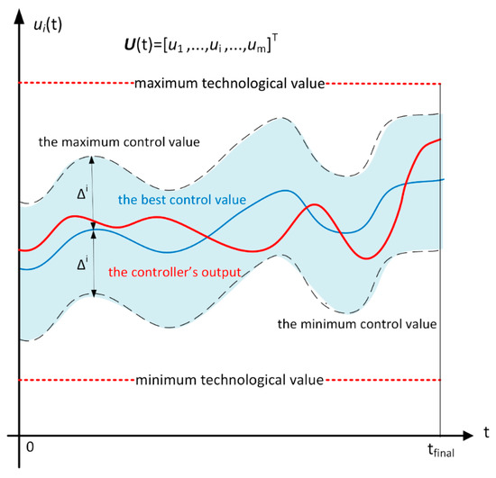
Controlling multi-agent systems (MASs) has attracted increased interest within the control community. Since the control challenge consists of the fact that each agent has limited local capabilities, our adopted solution is tailored so that a group of such entities works together and shares resources and information to fulfill a given task. In this work, we propose a coalitional control solution using the distributed model predictive control (DMPC) framework, suitable for a multi-agent system. The methodology has a switching mechanism that selects the best communication topology for the overall system. The proposed control algorithm was validated in simulation using a homogeneous vehicle platooning application with longitudinal dynamics. The available communication topologies were specifically tailored taking into account the information flow between adjacent vehicles. The obtained results show that when the platoon’s string stability is risked, the algorithm switches between different communication topologies. The resulting coalitions between vehicles ensure an increase in the overall stability of the entire system and prove the efficacy of our proposed methodology. Full article
Show Figures

Figure 1

Figure 1
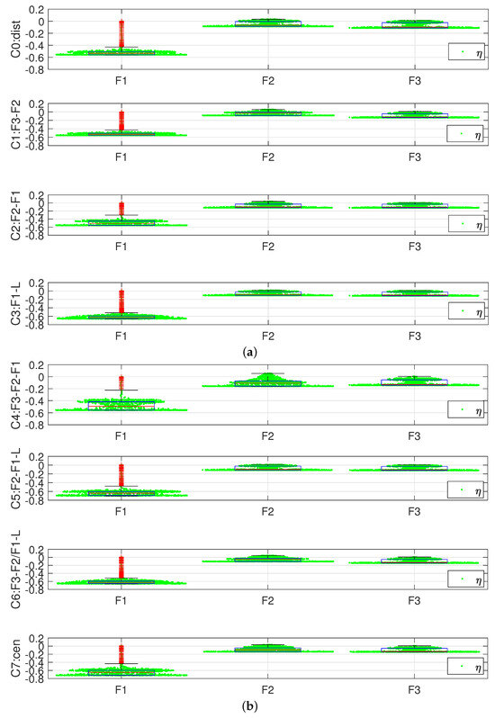
<p>Stability condition index. (<b>a</b>) Stability condition index for coalitions C0–C3. (<b>b</b>) Stability condition index for coalitions C4–C7.</p>
Full article ">Figure 2
<p>Velocity reference profiles used in Test 1, Test 2, and Test 3.</p>
Full article ">Figure 3
<p>Simulation results for the proposed C-DMPC strategy obtained in Test 1. (<b>a</b>) Test 1—velocity trajectories (1st subplot), position error trajectories in absolute value (2nd subplot), acceleration trajectories (3rd subplot), and control input trajectories (4th subplot). (<b>b</b>) Test 1—stability condition index (1st subplot), parameter <math display="inline"><semantics> <msub> <mi>N</mi> <mi>C</mi> </msub> </semantics></math> values (2nd subplot), and coalition selection (3rd subplot).</p>
Full article ">Figure 4
<p>Simulation results for the proposed C-DMPC strategy obtained in Test 2. (<b>a</b>) Test 2—velocity trajectories (1st subplot), position error trajectories in absolute value (2nd subplot), acceleration trajectories (3rd subplot), and control input trajectories (4th subplot). (<b>b</b>) Test 2—stability condition index (1st subplot), parameter <math display="inline"><semantics> <msub> <mi>N</mi> <mi>C</mi> </msub> </semantics></math> values (2nd subplot), and coalition selection (3rd subplot).</p>
Full article ">Figure 5
<p>Simulation results for the proposed C-DMPC strategy obtained in Test 3. (<b>a</b>) Test 3—velocity trajectories (1st subplot), position error trajectories in absolute value (2nd subplot), acceleration trajectories (3rd subplot), and control input trajectories (4th subplot). (<b>b</b>) Test 3—stability condition index (1st subplot), parameter <math display="inline"><semantics> <msub> <mi>N</mi> <mi>C</mi> </msub> </semantics></math> values (2nd subplot), and coalition selection (3rd subplot).</p>
Full article ">
2023

Jump to: 2024, 2022, 2021

17 pages, 7726 KiB  
Article
The Design and Development of a UAV’s Micro-Turbogenerator System and the Associated Control Testing Bench
by Tiberius-Florian Frigioescu, Gabriel Petre Badea, Mădălin Dombrovschi, Mihaela Raluca Condruz, Daniel-Eugeniu Crunțeanu and Grigore Cican
Electronics 2023, 12(24), 4904; https://doi.org/10.3390/electronics12244904 - 6 Dec 2023
Cited by 1 | Viewed by 1418
Abstract
A study on the possibility of integrating a micro-turbogenerator system into a multi-rotor UAV platform was performed along with a performance evaluation of the result. This paper presents the design and development of a micro-turbogenerator system constructed from commercially available components and the [...] Read more.
A study on the possibility of integrating a micro-turbogenerator system into a multi-rotor UAV platform was performed along with a performance evaluation of the result. This paper presents the design and development of a micro-turbogenerator system constructed from commercially available components and the associated test bench that was needed to validate the system. The goal of the micro-turbogenerator system was to replace the electrical power source (the batteries) of an experimental UAV. Substituting the electrical power source with a hybrid propulsion system has the potential to enhance the UAV’s endurance and functionality, rendering it more versatile and efficient. The hybrid propulsion system involves the use of a commercially available micro-gas turbine that propels an electric generator, supplying the required electrical power for the UAV’s electric propulsion system. Integrating this micro-turbogenerator system ensures a substantial increase in UAV endurance. The test bench was used to assess the performance of the micro-turbogenerator system and formulate a control law necessary for maintaining a balance between the power generated by the system and the power consumed by the UAV. The developed test bench yielded crucial data, including electric power, generated voltage, generator speed, and power consumption (simulating the UAV in this case). During the testing campaign, the variation in the main physical quantities involved in the command and control of the hybrid propulsion system was registered and analyzed. A total power of 700 W was obtained during the tests, which is the maximum that can be registered for maintaining a power of 25 V. Full article
Show Figures

Figure 1

Figure 1
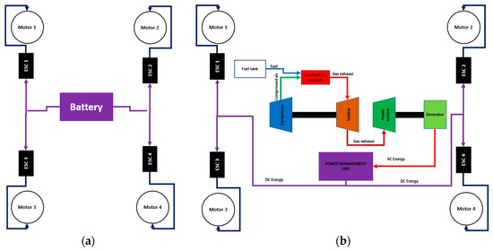
<p>Design scheme of the electrical (<b>a</b>) and hybrid system on a quadcopter (<b>b</b>).</p>
Full article ">Figure 2
<p>Three-dimensional CAD model of the testing bench.</p>
Full article ">Figure 3
<p>The complete testing bench configuration.</p>
Full article ">Figure 4
<p>Diagrams of the testing methods in Options A and B.</p>
Full article ">Figure 5
<p>Electrical diagram of the control system within the testing bench.</p>
Full article ">Figure 6
<p>Electrical diagram of the electric resistor system.</p>
Full article ">Figure 7
<p>Electrical diagram for an electric consumer—Option B.</p>
Full article ">Figure 8
<p>Flowchart diagram of the testing bench.</p>
Full article ">Figure 9
<p>(<b>a</b>) Starting position of the controller when the micromotor is in the idling stage. (<b>b</b>) The controller with the fuel throttler idling and the power throttler in the 50% consumer stage.</p>
Full article ">Figure 10
<p>Power consumption variation as a function of the nGB of the speed reducer gearbox. The red line was marked the point where the voltage was kept constant at a value of 25 V and the electric power was varied.</p>
Full article ">Figure 11
<p>Power consumption variation as a function of the micro-turbogenerator’s nG. The red line was marked the point where the voltage was kept constant at a value of 25 V and the electric power was varied.</p>
Full article ">Figure 12
<p>Voltage variation as a function of the nGB reductor gearbox’s speed. The red line was marked the point where the voltage was kept constant at a value of 25 V and the electric power was varied.</p>
Full article ">Figure 13
<p>Voltage variation as a function of nG micro-turbogenerator group’s speed. The red line was marked the point where the voltage was kept constant at a value of 25 V and the electric power was varied.</p>
Full article ">Figure 14
<p>nGB reductor gearbox speed variation as a function of the nG turbogenerator speed over the testing procedure. The red line was marked the point where the voltage was kept constant at a value of 25 V and the electric power was varied.</p>
Full article ">Figure 15
<p>Amperage variation as a function of the voltage over the testing procedure.</p>
Full article ">
32 pages, 5373 KiB  
Article
Optimization of Weight Matrices for the Linear Quadratic Regulator Problem Using Algebraic Closed-Form Solutions
by Daegyun Choi, Donghoon Kim and James D. Turner
Electronics 2023, 12(21), 4526; https://doi.org/10.3390/electronics12214526 - 3 Nov 2023
Cited by 1 | Viewed by 1110
Abstract
This work proposes an analytical gradient-based optimization approach to determine the optimal weight matrices that make the state and control input at the final time close to zero for the linear quadratic regulator problem. Most existing methodologies focused on regulating the diagonal elements [...] Read more.
This work proposes an analytical gradient-based optimization approach to determine the optimal weight matrices that make the state and control input at the final time close to zero for the linear quadratic regulator problem. Most existing methodologies focused on regulating the diagonal elements using only bio-inspired approaches or analytical approaches. The method proposed, contrarily, optimizes both diagonal and off-diagonal matrix elements based on the gradient. Moreover, by introducing a new variable composed of the steady-state and time-varying terms for the Riccati matrix and using the coordinate transformation for the state, one develops algebraic equationsbased closed-form solutions to generate the required states and numerical partial derivatives for an optimization strategy that does not require the computationally intensive numerical integration process. The authors test the algorithm with one- and two-degrees-of-freedom linear plant models, and it yields the weight matrices that successfully satisfy the pre-defined requirement, which is the norm of the augmented states less than 10−5. The results suggest the broad applicability of the proposed algorithm in science and engineering. Full article
Show Figures

Figure 1

Figure 1
<p>Conventional weight matrices selection procedure.</p>
Full article ">Figure 2
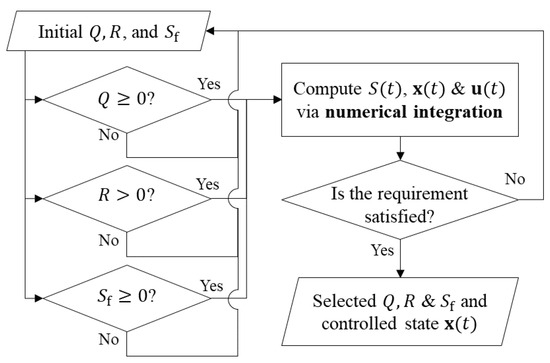
<p>Proposed weight matrices optimization procedure.</p>
Full article ">Figure 3
<p>System of the example problems. (<b>a</b>) 1 DOF. (<b>b</b>) 2 DOFs.</p>
Full article ">Figure 4
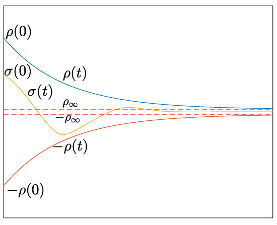
<p>State and control trajectories difference between the closed-form solutions and conventional approach. (<b>a</b>) 1 DOF. (<b>b</b>) 2 DOFs.</p>
Full article ">Figure 5
<p>History of the norm of the augmented state and the performance index (1 DOF).</p>
Full article ">Figure 6
<p>History of symmetric components of <span class="html-italic">Q</span> (1 DOF).</p>
Full article ">Figure 7
<p>History of symmetric components of <math display="inline"><semantics> <msub> <mi>S</mi> <mi mathvariant="normal">f</mi> </msub> </semantics></math> (1 DOF).</p>
Full article ">Figure 8
<p>History of symmetric components of <span class="html-italic">R</span> (1 DOF).</p>
Full article ">Figure 9
<p>Changes in state trajectories over iterations (1 DOF).</p>
Full article ">Figure 10
<p>Changes of optimal control trajectories over iterations (1 DOF).</p>
Full article ">Figure 11
<p>History of the norm of the augmented state and the performance index (2 DOFs).</p>
Full article ">Figure 12
<p>History of symmetric components of <span class="html-italic">Q</span> (2 DOFs).</p>
Full article ">Figure 13
<p>History of symmetric components of <math display="inline"><semantics> <msub> <mi>S</mi> <mi mathvariant="normal">f</mi> </msub> </semantics></math> (2 DOFs).</p>
Full article ">Figure 14
<p>History of symmetric components of <span class="html-italic">R</span> (2 DOFs).</p>
Full article ">Figure 15
<p>Changes in state trajectories over iterations (2 DOFs).</p>
Full article ">Figure 16
<p>Changes in optimal control trajectories over iterations (2 DOFs).</p>
Full article ">Figure A1
<p>History of the norm of the augmented state and the performance index (1 DOF).</p>
Full article ">Figure A2
<p>History of symmetric components of <span class="html-italic">Q</span> (1 DOF).</p>
Full article ">Figure A3
<p>History of symmetric components of <math display="inline"><semantics> <msub> <mi>S</mi> <mi mathvariant="normal">f</mi> </msub> </semantics></math> (1 DOF).</p>
Full article ">Figure A4
<p>History of symmetric components of <span class="html-italic">R</span> (1 DOF).</p>
Full article ">Figure A5
<p>Changes in state trajectories over iterations (1 DOF).</p>
Full article ">Figure A6
<p>Changes in optimal control trajectory over iterations (1 DOF).</p>
Full article ">Figure A7
<p>History of the norm of the augmented state and the performance index (2 DOFs).</p>
Full article ">Figure A8
<p>History of symmetric components of <span class="html-italic">Q</span> (2 DOFs).</p>
Full article ">Figure A9
<p>History of symmetric components of <math display="inline"><semantics> <msub> <mi>S</mi> <mi mathvariant="normal">f</mi> </msub> </semantics></math> (2 DOFs).</p>
Full article ">Figure A10
<p>History of symmetric components of <span class="html-italic">R</span> (2 DOFs).</p>
Full article ">Figure A11
<p>Changes of state trajectories over iterations (2 DOFs).</p>
Full article ">Figure A12
<p>Changes of optimal control trajectories over iterations (2 DOFs).</p>
Full article ">
16 pages, 7684 KiB  
Article
Slip Risk Prediction Using Intelligent Insoles and a Slip Simulator
by Shuo Xu, Md Javed Imtiaze Khan, Meysam Khaleghian and Anahita Emami
Electronics 2023, 12(21), 4393; https://doi.org/10.3390/electronics12214393 - 24 Oct 2023
Viewed by 1128
Abstract
Slip and fall accidents are the leading cause of injuries for all ages, and for fatal injuries in adults over 65 years. Various factors, such as floor surface conditions and contaminants, shoe tread patterns, and gait behavior, affect the slip risk. Moreover, the [...] Read more.
Slip and fall accidents are the leading cause of injuries for all ages, and for fatal injuries in adults over 65 years. Various factors, such as floor surface conditions and contaminants, shoe tread patterns, and gait behavior, affect the slip risk. Moreover, the friction between the shoe outsoles and the floor continuously changes as their surfaces undergo normal wear over time. However, continuous assessment of slip resistance is very challenging with conventional measurement techniques. This study addresses this challenge by introducing a novel approach that combines sensor fusion technology and machine learning techniques to create intelligent insoles designed for fall risk prediction. In addition, a state-of-the-art slip simulator, capable of mimicking the foot’s motion during a slip, was developed and utilized for the assessment of slipperiness between various shoes and floor surfaces. Data acquisition involved the collection of pressure data and three-axial accelerations using instrumented shoe insoles, complemented by friction coefficient measurements via the slip simulator. The collected dataset includes four types of shoes, three floor surfaces, and four surface conditions, including dry, wet, soapy, and oily. After preprocessing of the collected dataset, the simulator was used to train five different machine learning algorithms for slip risk classification. The trained algorithms provided promising results for slip risk prediction for different conditions, offering the potential to be employed in real-time slip risk prediction and safety enhancement. Full article
Show Figures

Figure 1

Figure 1
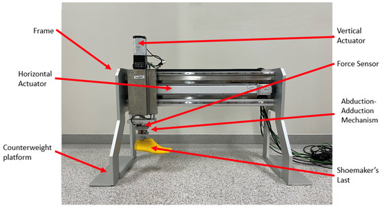
<p>Laboratory-type machine-based slip simulator measuring COF.</p>
Full article ">Figure 2
<p>CAD Model of the ankle mechanism (<b>a</b>) Ankle mechanism attached to the 3D-printed shoemaker’s last, (<b>b</b>) direction of screw hole for making plantar flexion and dorsiflexion angle, and (<b>c</b>) component required for making abduction and adduction angle.</p>
Full article ">Figure 3
<p>3D-printed instrumented insole with FSRs locations of US 9.5 men’s foot size.</p>
Full article ">Figure 4
<p>Surface conditions and footwear samples of Type A, B, C, D used in experiments.</p>
Full article ">Figure 5
<p>COF of the walking shoe on the mosaic floor.</p>
Full article ">Figure 6
<p>COFs for different floor and contamination conditions measured by the slip simulator.</p>
Full article ">Figure 7
<p>Foot pressure map of the Type A shoes while walking on the mosaic surface.</p>
Full article ">Figure 8
<p>Acceleration map of type A shoes during the walk on the mosaic surface.</p>
Full article ">Figure 9
<p>Power spectrum density during the walk on mosaic surface with Type A shoes.</p>
Full article ">Figure 10
<p>Power spectrum density of <math display="inline"> <semantics> <mrow> <msub> <mrow> <mi>a</mi> </mrow> <mrow> <mi>x</mi> </mrow> </msub> </mrow> </semantics> </math> during the walks (<b>a</b>) on multiple surfaces with Type A shoes in dry and oil conditions, and (<b>b</b>) on mosaic surface with all types of shoes in dry and oil conditions.</p>
Full article ">Figure 10 Cont.
<p>Power spectrum density of <math display="inline"> <semantics> <mrow> <msub> <mrow> <mi>a</mi> </mrow> <mrow> <mi>x</mi> </mrow> </msub> </mrow> </semantics> </math> during the walks (<b>a</b>) on multiple surfaces with Type A shoes in dry and oil conditions, and (<b>b</b>) on mosaic surface with all types of shoes in dry and oil conditions.</p>
Full article ">Figure 11
<p>(<b>a</b>) Acceleration correlation of the gait features to the COF, and (<b>b</b>) force correlation of the gait features to the COF.</p>
Full article ">Figure 11 Cont.
<p>(<b>a</b>) Acceleration correlation of the gait features to the COF, and (<b>b</b>) force correlation of the gait features to the COF.</p>
Full article ">Figure 12
<p>Performance of classifiers in a graphical way: (<b>a</b>) DT, (<b>b</b>) KNN, (<b>c</b>) RF, (<b>d</b>) SVM, and (<b>e</b>) LR.</p>
Full article ">Figure 12 Cont.
<p>Performance of classifiers in a graphical way: (<b>a</b>) DT, (<b>b</b>) KNN, (<b>c</b>) RF, (<b>d</b>) SVM, and (<b>e</b>) LR.</p>
Full article ">
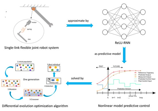
27 pages, 2349 KiB  
Article
Time-Series Machine Learning Techniques for Modeling and Identification of Mechatronic Systems with Friction: A Review and Real Application
by Samuel Ayankoso and Paweł Olejnik
Electronics 2023, 12(17), 3669; https://doi.org/10.3390/electronics12173669 - 30 Aug 2023
Cited by 6 | Viewed by 3303
Abstract
Developing accurate dynamic models for various systems is crucial for optimization, control, fault diagnosis, and prognosis. Recent advancements in information technologies and computing platforms enable the acquisition of input–output data from dynamical systems, resulting in a shift from physics-based methods to data-driven techniques [...] Read more.
Developing accurate dynamic models for various systems is crucial for optimization, control, fault diagnosis, and prognosis. Recent advancements in information technologies and computing platforms enable the acquisition of input–output data from dynamical systems, resulting in a shift from physics-based methods to data-driven techniques in science and engineering. This review examines different data-driven modeling approaches applied to the identification of mechanical and electronic systems. The approaches encompass various neural networks (NNs), like the feedforward neural network (FNN), convolutional neural network (CNN), long short-term memory (LSTM), transformer, and emerging machine learning (ML) techniques, such as the physics-informed neural network (PINN) and sparse identification of nonlinear dynamics (SINDy). The main focus is placed on applying these techniques to real-world problems. A real application is presented to demonstrate the effectiveness of different machine learning techniques, namely, FNN, CNN, LSTM, transformer, SINDy, and PINN, in data-driven modeling and the identification of a geared DC motor. The results show that the considered ML techniques (traditional and state-of-the-art methods) perform well in predicting the behavior of such a classic dynamical system. Furthermore, SINDy and PINN models stand out for their interpretability compared to the other data-driven models examined. Our findings explicitly show the satisfactory predictive performance of six different ML models while also highlighting their pros and cons, such as interpretability and computational complexity, using a real-world case study. The developed models have various applications and potential research areas are discussed. Full article
Show Figures

Figure 1

Figure 1
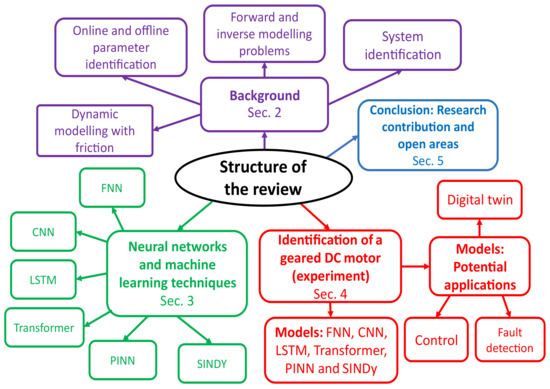
<p>A mind map of sections covered in this review.</p>
Full article ">Figure 2
<p>System identification steps.</p>
Full article ">Figure 3
<p>Approaches of dynamic modeling.</p>
Full article ">Figure 4
<p>A single neuron model.</p>
Full article ">Figure 5
<p>Illustration of gradient descent.</p>
Full article ">Figure 6
<p>An MLP network with three hidden layers (each neuron in the hidden layer is represented by <math display="inline"><semantics> <msub> <mi>h</mi> <mrow> <mi>i</mi> <mo>,</mo> <mi>j</mi> </mrow> </msub> </semantics></math>, where <span class="html-italic">i</span> is the neuron number and <span class="html-italic">j</span> is the hidden layer number).</p>
Full article ">Figure 7
<p>A one-dimensional CNN architecture for a regression task.</p>
Full article ">Figure 8
<p>Architecture of an RNN.</p>
Full article ">Figure 9
<p>LSTM cell.</p>
Full article ">Figure 10
<p>Transfomer block.</p>
Full article ">Figure 11
<p>A PINN approach based on physics-guided loss formulation.</p>
Full article ">Figure 12
<p>Block diagram of the control system with an incremental PWM step input, Arduino MEGA 2560 microcontroller, Pololu md07a high-power DC brushed motor driver, the object of control—DC motor SG555123000 10K with a gear and encoder; <math display="inline"><semantics> <mrow> <msub> <mover accent="true"> <mi>θ</mi> <mo>˙</mo> </mover> <mrow> <mi>r</mi> <mi>e</mi> <mi>f</mi> </mrow> </msub> <mrow> <mo>(</mo> <mi>t</mi> <mo>)</mo> </mrow> </mrow> </semantics></math>—the reference rotational velocity, <math display="inline"><semantics> <mrow> <msub> <mover accent="true"> <mi>θ</mi> <mo>˙</mo> </mover> <mrow> <mi>o</mi> <mi>s</mi> </mrow> </msub> <mrow> <mo>(</mo> <mi>t</mi> <mo>)</mo> </mrow> </mrow> </semantics></math>—the motor’s actual rotational velocity, <math display="inline"><semantics> <mrow> <mi>U</mi> <mo>(</mo> <mi>t</mi> <mo>)</mo> </mrow> </semantics></math>—the voltage input.</p>
Full article ">Figure 13
<p>Schematic diagram of a direct current motor.</p>
Full article ">Figure 14
<p>Angular speed prediction of different geared DC motor purely data-driven models after step-like increment of reference value.</p>
Full article ">Figure 15
<p>Angular speed prediction of different geared DC motor SINDy models after step-like increment of reference value.</p>
Full article ">Figure 16
<p>Prediction of the angular speed (<b>a</b>) and the armature current (<b>b</b>) of the geared DC motor PINN model after step-like increment of reference value.</p>
Full article ">Figure 16 Cont.
<p>Prediction of the angular speed (<b>a</b>) and the armature current (<b>b</b>) of the geared DC motor PINN model after step-like increment of reference value.</p>
Full article ">Figure 17
<p>Residual of each ML model.</p>
Full article ">
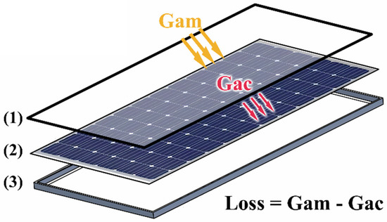
12 pages, 1889 KiB  
Article
A Predictive Current Control Strategy for a Medium-Voltage Open-End Winding Machine Drive
by Patricio Cataldo, Werner Jara, Javier Riedemann, Cristian Pesce, Iván Andrade and Rubén Pena
Electronics 2023, 12(5), 1070; https://doi.org/10.3390/electronics12051070 - 21 Feb 2023
Cited by 3 | Viewed by 1816
Abstract
This paper presents a medium-voltage drive based on an open-end winding induction machine supplied by a multilevel power converter topology. The power converter consists of cascaded two-level three-phase voltage source inverters (VSI) connected to each side of the machine windings and each VSI [...] Read more.
This paper presents a medium-voltage drive based on an open-end winding induction machine supplied by a multilevel power converter topology. The power converter consists of cascaded two-level three-phase voltage source inverters (VSI) connected to each side of the machine windings and each VSI is fed by an isolated DC supply. The topology has been previously reported in the literature as a sinusoidal pulse-width modulation operating in an open loop. In this work, a closed-loop model predictive control (MPC) strategy is proposed. MPC offers a much simpler method to control the power switches of the inverter compared to complex modulation strategies that are typically used in multilevel converters. Moreover, the advantage of reducing the common-mode voltage offered by the open-end winding configuration is fully exploited in this work. Simulation results are presented to validate the performance of the proposed topology and control method. Full article
Show Figures

Figure 1

Figure 1
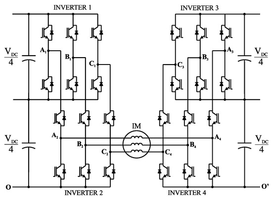
<p>Medium-voltage open-end winding induction motor drive.</p>
Full article ">Figure 2
<p>Space vector locations of the proposed topology.</p>
Full article ">Figure 3
<p>Diagram of the proposed current predictive control strategy for an open-end winding machine drive.</p>
Full article ">Figure 4
<p>Simulation results for the constant speed and change in the <span class="html-italic">q</span>-axis current. (<b>a</b>) Machine currents (<b>top</b>) and phase voltage (<b>bottom</b>); (<b>b</b>) <span class="html-italic">dq</span>-axis currents; (<b>c</b>) rotor speed (<b>top</b>) and common-mode voltage (<b>bottom</b>).</p>
Full article ">Figure 5
<p>Simulation results for the torque and change in the speed. (<b>a</b>) Machine currents (<b>top</b>) and phase voltage (<b>bottom</b>); (<b>b</b>) <span class="html-italic">dq</span>-axis currents; (<b>c</b>) rotor speed (<b>top</b>) and common-mode voltage (<b>bottom</b>).</p>
Full article ">Figure 5 Cont.
<p>Simulation results for the torque and change in the speed. (<b>a</b>) Machine currents (<b>top</b>) and phase voltage (<b>bottom</b>); (<b>b</b>) <span class="html-italic">dq</span>-axis currents; (<b>c</b>) rotor speed (<b>top</b>) and common-mode voltage (<b>bottom</b>).</p>
Full article ">Figure 6
<p>Comparison of MPC and SPWM. (<b>a</b>) Current THD as a function of the speed. (<b>b</b>) Torque ripple as a function of the speed.</p>
Full article ">Figure 7
<p>Average switching frequency as a function of the speed.</p>
Full article ">Figure 8
<p>Inverter efficiency as a function of the speed.</p>
Full article ">
17 pages, 5704 KiB  
Article
Clarifying Optimum Setting Temperatures for In-Flight Personal Air Conditioning System Considering Individual Thermal Sensitivity Characteristics
by Yuna Matsumoto, Manami Kanamaru, Phan Xuan Tan and Eiji Kamioka
Electronics 2023, 12(2), 371; https://doi.org/10.3390/electronics12020371 - 11 Jan 2023
Viewed by 1817
Abstract
The number of people who use airplanes has increased year by year. However, most passengers have a feeling of discomfort during a long-distance flight. One of the factors is the lack of temperature control in the cabin. If air conditioning control can be [...] Read more.
The number of people who use airplanes has increased year by year. However, most passengers have a feeling of discomfort during a long-distance flight. One of the factors is the lack of temperature control in the cabin. If air conditioning control can be adjusted to each passenger’s thermal sensation, the whole comfort in the cabin would be improved. Therefore, a personal air conditioning control method is required for airplanes. In order to implement personal air conditioning adapted to individual thermal sensation, this study proposes a seat-type air conditioning system that adjusts the temperature to each part of the body and aims to clarify the appropriate temperature setting in consideration of individual thermal sensation. As a result, the appropriate degree of temperature setting change was clarified based on the thermal sensation index. It was found that changing the temperature setting by 2.5 °C per scale of the thermal sensation improved the passenger’s comfort. Furthermore, people who tend to feel cold were found to be more sensitive to temperature changes. It is concluded that personalized air conditioning is possible based on individual thermal sensitivity characteristics. For prospects, it is desirable to study a system that automatically predicts the thermal sensation taking into account individual thermal sensitivity characteristics. Full article
Show Figures

Figure 1

Figure 1
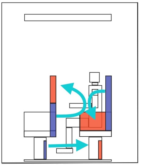
<p>Predicted airflow with inlets (red-colored) and outlets (blue-colored).</p>
Full article ">Figure 2
<p>Inlets (red-colored) and outlets (blue-colored) for personal air-conditioning system; outlets are positioned in six different areas.</p>
Full article ">Figure 3
<p>Flowchart of verification experiment.</p>
Full article ">Figure 4
<p>Relation between thermal comfort and thermal sensation.</p>
Full article ">Figure 5
<p>Experimental procedure.</p>
Full article ">Figure 6
<p>Thermal sensation evaluation index.</p>
Full article ">Figure 7
<p>Thermal comfort evaluation index.</p>
Full article ">Figure 8
<p>(<b>a</b>) Proposed air conditioning system and its experimental environment; (<b>b</b>) practical system used in verification experiment.</p>
Full article ">Figure 9
<p>Verification experiment environment.</p>
Full article ">Figure 10
<p>Subject’s clothes.</p>
Full article ">Figure 11
<p>Average thermal sensation for each part of the body.</p>
Full article ">Figure 12
<p>Average thermal comfort for each part of the body.</p>
Full article ">Figure 13
<p>Comparison of thermal sensation and thermal comfort, and tendency to feel hot and cold.</p>
Full article ">

2022

Jump to: 2024, 2023, 2021

14 pages, 5469 KiB  
Article
Stability Analysis for Single-Lane Traffic with a Relay Controller in a Closed Loop
by Monica Patrascu and Vlad Constantinescu
Electronics 2023, 12(1), 5; https://doi.org/10.3390/electronics12010005 - 20 Dec 2022
Cited by 1 | Viewed by 1961
Abstract
Rule-based relay controllers are common in single-lane urban traffic control systems and introduce significant nonlinearity. In this paper, we analyze the closed-loop stability for a traffic process with a relay controller and negative feedback, with respect to several time delays present in the [...] Read more.
Rule-based relay controllers are common in single-lane urban traffic control systems and introduce significant nonlinearity. In this paper, we analyze the closed-loop stability for a traffic process with a relay controller and negative feedback, with respect to several time delays present in the plant. First, we derive models for the road segment and the controller. Second, we investigate the system stability based on describing the function analysis. Finally, we present the numerical results. Full article
Show Figures

Figure 1

Figure 1
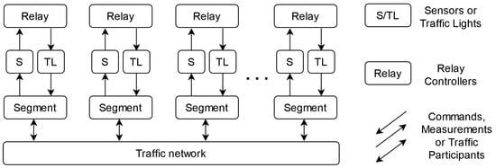
<p>Structure of the decentralized control system for the traffic network.</p>
Full article ">Figure 2
<p>Road segment representation.</p>
Full article ">Figure 3
<p>Model structure for vehicle load on a single-lane road segment.</p>
Full article ">Figure 4
<p>Traffic control system structure for a single-lane road segment.</p>
Full article ">Figure 5
<p>Response of the traffic control system for a single-lane road segment: setpoint <math display="inline"><semantics> <mrow> <msub> <mi>R</mi> <mn>0</mn> </msub> <mrow> <mo>(</mo> <mi>t</mi> <mo>)</mo> </mrow> <mo>=</mo> <mn>10</mn> </mrow> </semantics></math> (vehicles, blue), output <math display="inline"><semantics> <mrow> <mi>R</mi> <mo>(</mo> <mi>t</mi> <mo>)</mo> </mrow> </semantics></math> (vehicles, red), and command <math display="inline"><semantics> <mrow> <mi>U</mi> <mo>(</mo> <mi>t</mi> <mo>)</mo> <mo>=</mo> <mo>−</mo> <mn>1</mn> </mrow> </semantics></math> for green phase (vehicles are released) or <math display="inline"><semantics> <mrow> <mi>U</mi> <mo>(</mo> <mi>t</mi> <mo>)</mo> <mo>=</mo> <mn>0</mn> </mrow> </semantics></math> for red phase (vehicles are received).</p>
Full article ">Figure 6
<p>Nonlinear components.</p>
Full article ">Figure 7
<p>Limit cycle stability.</p>
Full article ">Figure 8
<p>Behavior for setpoint 40 vehicles, where <math display="inline"><semantics> <mrow> <mi>n</mi> <mo>=</mo> <mn>1</mn> </mrow> </semantics></math>, <math display="inline"><semantics> <mrow> <mi>n</mi> <mo>=</mo> <mn>3</mn> </mrow> </semantics></math>, and <math display="inline"><semantics> <mrow> <msub> <mi>τ</mi> <mi>c</mi> </msub> <mo>=</mo> <mn>5</mn> </mrow> </semantics></math> s.</p>
Full article ">Figure 9
<p>Frequency response of the linear component: stable for <math display="inline"><semantics> <mrow> <mrow> <mo>(</mo> <mi>n</mi> <mo>,</mo> <msub> <mi>τ</mi> <mi>c</mi> </msub> <mo>)</mo> </mrow> <mo>∈</mo> <mrow> <mo>{</mo> <mrow> <mo>(</mo> <mn>1</mn> <mo>,</mo> <mn>5</mn> <mo>)</mo> </mrow> <mo>,</mo> <mrow> <mo>(</mo> <mn>1.5</mn> <mo>,</mo> <mn>5</mn> <mo>)</mo> </mrow> <mo>,</mo> <mrow> <mo>(</mo> <mn>2</mn> <mo>,</mo> <mn>5</mn> <mo>)</mo> </mrow> <mo>}</mo> </mrow> </mrow> </semantics></math> and unstable for <math display="inline"><semantics> <mrow> <mrow> <mo>(</mo> <mi>n</mi> <mo>,</mo> <msub> <mi>τ</mi> <mi>c</mi> </msub> <mo>)</mo> </mrow> <mo>∈</mo> <mrow> <mo>{</mo> <mrow> <mo>(</mo> <mn>1</mn> <mo>,</mo> <mn>60</mn> <mo>)</mo> </mrow> <mo>,</mo> <mrow> <mo>(</mo> <mn>4</mn> <mo>,</mo> <mn>30</mn> <mo>)</mo> </mrow> <mo>,</mo> <mrow> <mo>(</mo> <mn>5</mn> <mo>,</mo> <mn>40</mn> <mo>)</mo> </mrow> <mo>}</mo> </mrow> </mrow> </semantics></math>.</p>
Full article ">Figure 10
<p>Single-lane road segments in a network, showing structure and time responses.</p>
Full article ">
24 pages, 10108 KiB  
Article
A New Decentralized PQ Control for Parallel Inverters in Grid-Tied Microgrids Propelled by SMC-Based Buck–Boost Converters
by Ali M. Jasim, Basil H. Jasim and Bogdan-Constantin Neagu
Electronics 2022, 11(23), 3917; https://doi.org/10.3390/electronics11233917 - 27 Nov 2022
Cited by 16 | Viewed by 2923
Abstract
Nowadays, the microgrid (MG) concept is regarded as an efficient approach to incorporating renewable generation resources into distribution networks. However, managing power flows to distribute load power among distribution generators (DGs) remains a critical focus, particularly during peak demand. The purpose of this [...] Read more.
Nowadays, the microgrid (MG) concept is regarded as an efficient approach to incorporating renewable generation resources into distribution networks. However, managing power flows to distribute load power among distribution generators (DGs) remains a critical focus, particularly during peak demand. The purpose of this paper is to control the adopted grid-tied MG performance and manage the power flow from/to the parallel DGs and the main grid using discrete-time active/reactive power (PQ) control based on digital proportional resonant (PR) controllers. The PR controller is used to eliminate harmonics by acting as a digital infinite-impulse response (IIR) filter with a high gain at the resonant frequency. Additionally, the applied PR controller has fast reference signal tracking, responsiveness to grid frequency drift, and no steady-state error. Moreover, this paper describes the application of robust nonlinear sliding mode control (SMC)-technique-based buck–boost (BB) converters. The sliding adaptive control scheme is applied to prevent the output voltage error that occurs during DG failure, load variations, or system parameter changes. This paper deals with two distinct case studies. The first one focuses on applying the proposed control for two parallel DGs with and without load-changing conditions. In the latter case, the MG is expanded to include five DGs (with and without DG failure). The proposed control technique has been compared with the droop control and model predictive control (MPC) techniques. As demonstrated by the simulation results in MATLAB software, the proposed method outperformed the others in terms of both performance analysis and the ability to properly share power between parallel DGs and the utility grid. Full article
Show Figures

Figure 1

Figure 1
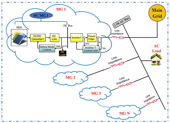
<p>Parallel decentralized MGs.</p>
Full article ">Figure 2
<p>Three-phase two-level inverter output voltage vectors.</p>
Full article ">Figure 3
<p>The two-DGs-based adopted MG system.</p>
Full article ">Figure 4
<p>The SMC process works (<b>1</b>): (<b>a</b>) reaching phase, (<b>b</b>) sliding phase; trajectory movement according to hitting (<b>2</b>) and existence (<b>3</b>) conditions.</p>
Full article ">Figure 5
<p>A schematic diagram of a PID-based sliding mode voltage-controlled BB converter.</p>
Full article ">Figure 6
<p>The proposed control technique of one inverter.</p>
Full article ">Figure 7
<p>The magnitude and phase response of the designed (<b>a</b>) resonance filter and (<b>b</b>) PR controller.</p>
Full article ">Figure 8
<p>(<b>a</b>) The representation block diagram scheme of MPC and (<b>b</b>) the MPC flowchart.</p>
Full article ">Figure 9
<p>The input and output voltages of the BB converters’ operation: (<b>a</b>) buck converters, (<b>b</b>) boost converters, and (<b>c</b>) the first converter is buck and the second is boost.</p>
Full article ">Figure 10
<p>Individual DG power flow control using MPC.</p>
Full article ">Figure 11
<p>Individual DG power flow control using the proposed PQ control: (<b>a</b>) active power and (<b>b</b>) reactive power.</p>
Full article ">Figure 12
<p>Active and reactive net power flows to the grid using PQ-control-based digital PR controllers.</p>
Full article ">Figure 13
<p>AC common bus frequency using the proposed technique.</p>
Full article ">Figure 14
<p>AC common bus current and voltage using the proposed technique: (<b>a</b>) current and (<b>b</b>) voltage signal.</p>
Full article ">Figure 15
<p>Individual DG power flow control using the proposed technique under changing load conditions: (<b>a</b>) active power and (<b>b</b>) reactive power.</p>
Full article ">Figure 16
<p>Active and reactive net power flows to the grid using the proposed technique under changing load conditions.</p>
Full article ">Figure 17
<p>AC common bus frequency using the proposed technique under changing load conditions.</p>
Full article ">Figure 18
<p>AC common bus current and voltage using the proposed technique under changing load conditions: (<b>a</b>) current and (<b>b</b>) voltage signal.</p>
Full article ">Figure 19
<p>Individual DG power flow control under the second case study without an outage DG: (<b>a</b>) active power and (<b>b</b>) reactive power.</p>
Full article ">Figure 20
<p>Individual DG power flow control under the second case study with an outage third DG: (<b>a</b>) active power and (<b>b</b>) reactive power.</p>
Full article ">Figure 21
<p>Active and reactive net power flows to the grid under the second case study without DG outage or with a third DG outage.</p>
Full article ">
27 pages, 824 KiB  
Article
Bacterial Memetic Algorithm for Asymmetric Capacitated Vehicle-Routing Problem
by Ákos Holló-Szabó and János Botzheim
Electronics 2022, 11(22), 3758; https://doi.org/10.3390/electronics11223758 - 16 Nov 2022
Cited by 3 | Viewed by 1685
Abstract
The vehicle-routing problem (VRP) has many variants, including the most accurate models of real-life transportation tasks, making it one of the most important mathematical problems in the field of logistics. Our goal was to design an algorithm that can race against the most [...] Read more.
The vehicle-routing problem (VRP) has many variants, including the most accurate models of real-life transportation tasks, making it one of the most important mathematical problems in the field of logistics. Our goal was to design an algorithm that can race against the most recent solutions for VRP and capacitated VRP (CVRP), while also being applicable to real-life models with simulations of real transports. Our algorithm is a variant of the bacterial memetic algorithm (BMA), which we improve upon with novel operators and better methods for manual parameter optimization. The key to our performance is a balanced mixture of the global search of evolutionary algorithms, local search of 2-OPT variants, and the pseudo-global search of probabilistic construction algorithms. Our algorithm benefits from the advantages of all three methods resulting in fast convergence and avoidance of global minima. This is the first time BMA is applied for VRP, meaning that we had to adapt the method for the new problem. We compare our method with some of the most-used methods for VRP on the ABEFMP 1995 dataset. We provide comparison results with the coronavirus herd immunity optimizer, genetic algorithm, hybridization of genetic algorithm with neighborhood search, firefly algorithm, enhanced firefly algorithm, ant colony optimization, and variable neighborhood search. Our algorithm performed better on all data instances, yielding at least a 30% improvement. We present our best result on the Belgium 2017 dataset for future reference. Finally, we show that our algorithm is capable of handling real-life models. Here we are also illustrating the significance of the different parameters. Full article
Show Figures

Figure 1

Figure 1
<p>K-Opt Algorithm Family. Here, the dashed lines represent the new edges of the cycle created by the different operators.</p>
Full article ">Figure 2
<p>Genetic algorithm.</p>
Full article ">Figure 3
<p>Crossover step of genetic algorithm. We marked the elements inherited from the primary parent by underlining the values. We only demonstrate the basic idea, there are hundreds of other known crossover operators.</p>
Full article ">Figure 4
<p>Bacterial memetic algorithm.</p>
Full article ">Figure 5
<p>Chromosome representation. In the first representation, the end of segments are represented by wider separator lines. In the second representation, star symbols represent the inserted break points. Break points are replaced by numbers in the final design.</p>
Full article ">Figure 6
<p>Bacterial mutation. The values of the selected segment in each specimen are underlined. The white arrow represents that the original specimen is overwritten by the best clone.</p>
Full article ">Figure 7
<p>Boxplot of scenarios on the A-n32-k5 task of ABEFMP.</p>
Full article ">Figure 8
<p>Boxplot of scenarios on the A-n34-k5 task of ABEFMP.</p>
Full article ">Figure 9
<p>Boxplot of scenarios on the A-n39-k6 task of ABEFMP.</p>
Full article ">Figure 10
<p>Boxplot of scenarios on the A-n45-k7 task of ABEFMP.</p>
Full article ">Figure 11
<p>Boxplot of scenarios on the A-n48-k7 task of ABEFMP.</p>
Full article ">Figure 12
<p>Boxplot of scenarios on the A-n55-k9 task of ABEFMP.</p>
Full article ">Figure 13
<p>Boxplot of scenarios on the A-n60-k9 task of ABEFMP.</p>
Full article ">Figure 14
<p>Boxplot of scenarios on the A-n69-k9 task of ABEFMP.</p>
Full article ">Figure 15
<p>Boxplot of scenarios on the A-n80-k10 task of ABEFMP.</p>
Full article ">Figure 16
<p>Progress of population of the best run on Belgium 2017 dataset.</p>
Full article ">Figure 17
<p>All 10 runs on Belgium 2017 dataset.</p>
Full article ">Figure 18
<p>All 10 runs on Belgium 2017 dataset, magnified.</p>
Full article ">Figure 19
<p>Boxplot of 10 runs on Belgium 2017 dataset.</p>
Full article ">Figure 20
<p>Scenarios on the Hungarian dataset.</p>
Full article ">Figure 21
<p>Boxplot of scenarios on the Hungarian dataset.</p>
Full article ">
19 pages, 8878 KiB  
Article
A Fuzzy Entropy-Based Thematic Classification Method Aimed at Improving the Reliability of Thematic Maps in GIS Environments
by Barbara Cardone and Ferdinando Di Martino
Electronics 2022, 11(21), 3509; https://doi.org/10.3390/electronics11213509 - 28 Oct 2022
Cited by 3 | Viewed by 1337
Abstract
Thematic maps of spatial data are constructed by using standard thematic classification methods that do not allow management of the uncertainty of classification and, consequently, evaluation of the reliability of the resulting thematic map. We propose a novel fuzzy-based thematic classification method applied [...] Read more.
Thematic maps of spatial data are constructed by using standard thematic classification methods that do not allow management of the uncertainty of classification and, consequently, evaluation of the reliability of the resulting thematic map. We propose a novel fuzzy-based thematic classification method applied to construct thematic maps in Geographical Information Systems. An initial fuzzy partition of the domain of the features of the spatial dataset is constructed using triangular fuzzy numbers; our method finds an optimal fuzzy partition evaluating the fuzziness of the fuzzy sets by using a fuzzy entropy measure. An assessment of the reliability of the final thematic map is performed according to the fuzziness of the fuzzy sets. We implement our method on a GIS framework, testing it on various vector and image spatial datasets. The results of these tests confirm that our thematic classification method provide thematic maps with a higher reliability with respect to that obtained through fuzzy partitions constructed by expert users. Full article
Show Figures

Figure 1

Figure 1
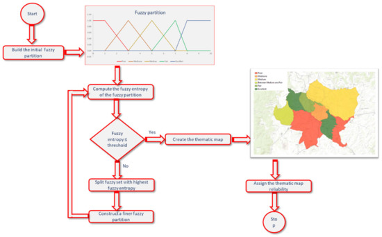
<p>Schema of the Thematic Fuzzy Entropy Partition method (TFEP).</p>
Full article ">Figure 2
<p>Example of fuzzy partition built using fuzzy numbers.</p>
Full article ">Figure 3
<p>Shannon’s Entropy function.</p>
Full article ">Figure 4
<p>Example of fuzzy partition of the domain [0%,100%] with 4 fuzzy sets.</p>
Full article ">Figure 5
<p>Final fuzzy partition with 5 fuzzy sets.</p>
Full article ">Figure 6
<p>The study area: the municipalities of the province of Florence (Italy).</p>
Full article ">Figure 7
<p>The initial fuzzy partition given by 3 fuzzy numbers.</p>
Full article ">Figure 8
<p>The thematic map of the number of inhabitants in residential buildings using the initial fuzzy partition.</p>
Full article ">Figure 9
<p>The new fuzzy partition given by 4 fuzzy numbers.</p>
Full article ">Figure 10
<p>Final thematic map of the number of inhabitants in residential buildings.</p>
Full article ">Figure 11
<p>The study area: satellite image of the NDVI index on the municipality of Naples (Italy).</p>
Full article ">Figure 12
<p>The initial fuzzy partition of the NDVI index given by 4 fuzzy numbers.</p>
Full article ">Figure 13
<p>The thematic map of the NDVI index using the initial fuzzy partition.</p>
Full article ">Figure 14
<p>The second fuzzy partition of NDVI given by 5 fuzzy numbers.</p>
Full article ">Figure 15
<p>The thematic map of the NDVI index using fuzzy partition in <a href="#electronics-11-03509-f014" class="html-fig">Figure 14</a>.</p>
Full article ">Figure 16
<p>The third fuzzy partition of NDVI given by 6 fuzzy numbers.</p>
Full article ">Figure 17
<p>The final thematic map of the NDVI index.</p>
Full article ">Figure 18
<p>Trend of the map-reliability gain.</p>
Full article ">
16 pages, 2650 KiB  
Article
Trend Prediction Based on Multi-Modal Affective Analysis from Social Networking Posts
by Kazuyuki Matsumoto, Reishi Amitani, Minoru Yoshida and Kenji Kita
Electronics 2022, 11(21), 3431; https://doi.org/10.3390/electronics11213431 - 23 Oct 2022
Cited by 2 | Viewed by 1590
Abstract
This paper propose a method to predict the stage of buzz-trend generation by analyzing the emotional information posted on social networking services for multimodal information, such as posted text and attached images, based on the content of the posts. The proposed method can [...] Read more.
This paper propose a method to predict the stage of buzz-trend generation by analyzing the emotional information posted on social networking services for multimodal information, such as posted text and attached images, based on the content of the posts. The proposed method can analyze the diffusion scale from various angles, using only the information at the time of posting, when predicting in advance and the information of time error, when used for posterior analysis. Specifically, tweets and reply tweets were converted into vectors using the BERT general-purpose language model that was trained in advance, and the attached images were converted into feature vectors using a trained neural network model for image recognition. In addition, to analyze the emotional information of the posted content, we used a proprietary emotional analysis model to estimate emotions from tweets, reply tweets, and image features, which were then added to the input as emotional features. The results of the evaluation experiments showed that the proposed method, which added linguistic features (BERT vectors) and image features to tweets, achieved higher performance than the method using only a single feature. Although we could not observe the effectiveness of the emotional features, the more emotions a tweet and its reply match had, the more empathy action occurred and the larger the like and RT values tended to be, which could ultimately increase the likelihood of a tweet going viral. Full article
Show Figures

Figure 1

Figure 1
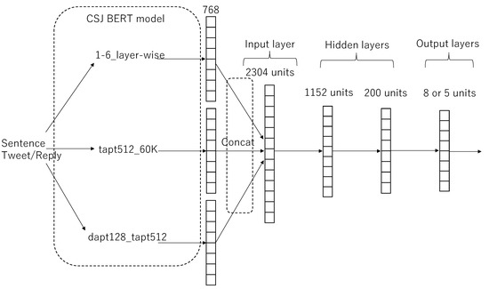
<p>Emotion estimation networks for estimating eight emotions/five emotions.</p>
Full article ">Figure 2
<p>Emotion estimation network that outputs two types of emotion classes based on multi-task learning.</p>
Full article ">Figure 3
<p>Distribution of number of likes and retweets; (<b>a</b>) number of likes (over100), (<b>b</b>) number of RTs (over100), (<b>c</b>) number of likes (under100), (<b>d</b>) number of RTs (under100).</p>
Full article ">Figure 4
<p>Relation between like/RT and feature vectors of tweets and replies. (<b>a</b>) Relation of sim<sub>tw8,rp8</sub> and like, (<b>b</b>) Relation of sim<sub>tw8,rp8,</sub> RT, (<b>c</b>) Relation of sim<sub>tw5,rp5,</sub> like, (<b>d</b>) Relation of sim<sub>tw5,rp5,</sub> RT, (<b>e</b>) Relation of sim<sub>twh,rph,</sub> like, (<b>f</b>) Relation of sim<sub>twh,rph,</sub> RT<sub>,</sub> like, (<b>g</b>) Relation of sim<sub>twb,rpb,</sub> like, (<b>h</b>) Relation of sim<sub>twb,rpb,</sub> RT.</p>
Full article ">Figure 5
<p>Relationship between RT, like, and emotion vectors (8 emotions).</p>
Full article ">Figure 6
<p>Relationship between RT, like, and tweet and reply emotions; (<b>a</b>) eight emotions and likes, (<b>b</b>) eight emotions and RTs, (<b>c</b>) five emotions and likes, (<b>d</b>) five emotions and RTs (the horizontal label indicates the quartile range label of like/RT).</p>
Full article ">
19 pages, 9899 KiB  
Article
Methods for Model Complexity Reduction for the Nonlinear Calibration of Amplifiers Using Volterra Kernels
by Francesco Centurelli, Pietro Monsurrò, Giuseppe Scotti, Pasquale Tommasino and Alessandro Trifiletti
Electronics 2022, 11(19), 3067; https://doi.org/10.3390/electronics11193067 - 26 Sep 2022
Cited by 1 | Viewed by 1605
Abstract
Volterra models allow modeling nonlinear dynamical systems, even though they require the estimation of a large number of parameters and have, consequently, potentially large computational costs. The pruning of Volterra models is thus of fundamental importance to reduce the computational costs of nonlinear [...] Read more.
Volterra models allow modeling nonlinear dynamical systems, even though they require the estimation of a large number of parameters and have, consequently, potentially large computational costs. The pruning of Volterra models is thus of fundamental importance to reduce the computational costs of nonlinear calibration, and improve stability and speed, while preserving accuracy. Several techniques (LASSO, DOMP and OBS) and their variants (WLASSO and OBD) are compared in this paper for the experimental calibration of an IF amplifier. The results show that Volterra models can be simplified, yielding models that are 4–5 times sparser, with a limited impact on accuracy. About 6 dB of improved Error Vector Magnitude (EVM) is obtained, improving the dynamic range of the amplifiers. The Symbol Error Rate (SER) is greatly reduced by calibration at a large input power, and pruning reduces the model complexity without hindering SER. Hence, pruning allows improving the dynamic range of the amplifier, with almost an order of magnitude reduction in model complexity. We propose the OBS technique, used in the neural network field, in conjunction with the better known DOMP technique, to prune the model with the best accuracy. The simulations show, in fact, that the OBS and DOMP techniques outperform the others, and OBD, LASSO and WLASSO are, in turn, less efficient. A methodology for pruning in the complex domain is described, based on the Frisch–Waugh–Lovell (FWL) theorem, to separate the linear and nonlinear sections of the model. This is essential because linear models are used for equalization and cannot be pruned to preserve model generality vis-a-vis channel variations, whereas nonlinear models must be pruned as much as possible to minimize the computational overhead. This methodology can be extended to models other than the Volterra one, as the only conditions we impose on the nonlinear model are that it is feedforward and linear in the parameters. Full article
Show Figures

Figure 1

Figure 1
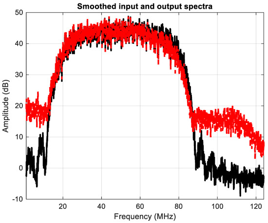
<p>Input (black) and output (red) spectra. Spectral regrowth is clearly visible at the output.</p>
Full article ">Figure 2
<p>EVM (top) and SER (bottom) after equalization with 9 linear coefficients and offset correction. Transmission errors are evident, and the EVM is too large.</p>
Full article ">Figure 3
<p>Received constellation after equalization. The QAM-64 constellation should form a square of 8 dots per dimension. Noise is limited (the central dots are small), but heavy distortion occurs at the diagonal corners, due to nonlinear effects. Such distortions produce transmission errors, as shown in <a href="#electronics-11-03067-f002" class="html-fig">Figure 2</a>.</p>
Full article ">Figure 4
<p>EVM (top) and SER (bottom) after calibration with 72 coefficients. Symbol errors are no longer present, but model complexity significantly increased.</p>
Full article ">Figure 5
<p>Received constellation after calibration. The shape of the constellation has significantly improved, though some nonlinear errors are still present at the four diagonal corners of the constellation, where amplitude is maximum.</p>
Full article ">Figure 6
<p>Accuracy vs. complexity for the five pruning techniques. OBS and DOMP outperform all the others. LASSO is the least efficient, whereas OBD is not bad for relatively large models. WLASSO is significantly better than LASSO, though still inefficient with respect to OBS and DOMP.</p>
Full article ">Figure 7
<p>Zoom for OBS vs. DOMP, the two most promising pruning techniques. The two curves intersect each other, so that neither OBS nor DOMP are optimal by themselves. However, their combined use allows finding the best approximation of the optimal complexity-accuracy trade-off.</p>
Full article ">Figure 8
<p>SER and EVM after pruning to 22 coefficients. The EVM increase is minimal, and SER is still zero, despite the fact that the nonlinear coefficients are decreased from 62 to just 12, close to an 80% reduction in complexity.</p>
Full article ">Figure 9
<p>Constellation after pruning with 22 coefficients.</p>
Full article ">Figure 10
<p>EVM vs. the number of symbols in the train dataset. Convergence is achieved after about 1500 samples. EVM is computed over both the train and test datasets, where the train dataset includes the first symbols, used for training, and the test dataset includes the remaining symbols, used to compute the EVM but not to estimate the model coefficients.</p>
Full article ">Figure 11
<p>EVM of the equalization (black), calibration (red) and pruned (blue) models as a function of the input power level. Calibration allows reducing EVM by a factor 2, and pruning has limited impact on accuracy, though a very large one on model complexity (with a reduction from 62 to 12 nonlinear model coefficients).</p>
Full article ">
15 pages, 4902 KiB  
Article
A Piece-Wise Linear Model-Based Algorithm for the Identification of Nonlinear Models in Real-World Applications
by Claudio Carnevale, Lucia Sangiorgi, Renata Mansini and Roberto Zanotti
Electronics 2022, 11(17), 2770; https://doi.org/10.3390/electronics11172770 - 2 Sep 2022
Cited by 2 | Viewed by 1538
Abstract
In this work, a data-driven approach for the identification of a piece-wise linear model for nitrogen oxide daily concentration simulation is presented and applied. The model has been identified by using daily measured concentrations, meteorological variables, and emission levels estimated starting from the [...] Read more.
In this work, a data-driven approach for the identification of a piece-wise linear model for nitrogen oxide daily concentration simulation is presented and applied. The model has been identified by using daily measured concentrations, meteorological variables, and emission levels estimated starting from the results contained in suitable emission databases. We propose an innovative methodology that jointly optimizes clustering and parameter identification. The procedure has been applied considering data from the Milan (Italy) metropolitan area. The methodology has been compared with two state-of-the-art approaches based on a two-step, cluster-based algorithm and on Hammerstein–Wiener models. The results show how, in the presented application, the devised approach ensures better performance with respect to the two literature methods, both in terms of statistical indexes (correlation, normalized mean absolute error) and in terms of problem-specific metrics (hit ratio, false alarm). For this reason, the approach can be considered suitable to be used in the definition of optimal emission control strategies. Full article
Show Figures

Figure 1

Figure 1
<p>Index values (ordinate axis) of ARX model for (<math display="inline"><semantics> <mrow> <mi>K</mi> <mo>=</mo> <mn>1</mn> </mrow> </semantics></math>) with <math display="inline"><semantics> <mrow> <msub> <mi>n</mi> <mi>a</mi> </msub> <mo>=</mo> <msub> <mi>n</mi> <mi>l</mi> </msub> <mo>=</mo> <mn>1</mn> <mo>…</mo> <mn>4</mn> </mrow> </semantics></math> (abscissa axis). (<b>a</b>) Normalized Mean Absolute Error (NMAE); (<b>b</b>) Correlation Coefficient; (<b>c</b>) Hit Ratio; (<b>d</b>) False Alarm; (<b>e</b>) True Skill Score (TSS).</p>
Full article ">Figure 2
<p>Index values (ordinate axis) of the 5 compared methods for <math display="inline"><semantics> <mrow> <mi>K</mi> <mo>=</mo> <mn>1</mn> <mo>…</mo> <mn>10</mn> </mrow> </semantics></math> (abscissa axis) when <math display="inline"><semantics> <mrow> <msub> <mi>n</mi> <mi>a</mi> </msub> <mo>=</mo> <msub> <mi>n</mi> <mi>l</mi> </msub> <mo>=</mo> <mn>1</mn> </mrow> </semantics></math>. (<b>a</b>) Normalized Mean Absolute Error (NMAE); (<b>b</b>) Correlation Coefficient; (<b>c</b>) Hit Ratio; (<b>d</b>) False Alarm; (<b>e</b>) True Skill Score (TSS).</p>
Full article ">Figure 3
<p>Boxplot of coordinate 1 (<math display="inline"><semantics> <mrow> <mi>y</mi> <mo>(</mo> <mi>t</mi> <mo>−</mo> <mn>1</mn> <mo>)</mo> </mrow> </semantics></math>, NO<math display="inline"><semantics> <msub> <mrow/> <mn>2</mn> </msub> </semantics></math> concentration at time <math display="inline"><semantics> <mrow> <mi>t</mi> <mo>−</mo> <mn>1</mn> </mrow> </semantics></math>) of the centroid [<math display="inline"><semantics> <mi mathvariant="sans-serif">μ</mi> </semantics></math>g/m<math display="inline"><semantics> <msup> <mrow/> <mn>3</mn> </msup> </semantics></math>].</p>
Full article ">Figure 4
<p>Boxplot of coordinate 2 (<math display="inline"><semantics> <mrow> <msub> <mi>u</mi> <mn>1</mn> </msub> <mrow> <mo>(</mo> <mi>t</mi> <mo>)</mo> </mrow> </mrow> </semantics></math>, NO<math display="inline"><semantics> <msub> <mrow/> <mi>x</mi> </msub> </semantics></math> emissions at time <span class="html-italic">t</span>) of the centroid [kg/d/m <math display="inline"><semantics> <msup> <mrow/> <mn>2</mn> </msup> </semantics></math>].</p>
Full article ">Figure 5
<p>Boxplot of coordinate 3 (<math display="inline"><semantics> <mrow> <msub> <mi>u</mi> <mn>2</mn> </msub> <mrow> <mo>(</mo> <mi>t</mi> <mo>)</mo> </mrow> </mrow> </semantics></math>, daily mean temperature at time <span class="html-italic">t</span>) of the centroid <math display="inline"><semantics> <mrow> <mo>[</mo> <mi>C</mi> <mo>]</mo> </mrow> </semantics></math>.</p>
Full article ">Figure 6
<p>Boxplot of coordinate 4 (<math display="inline"><semantics> <mrow> <msub> <mi>u</mi> <mn>3</mn> </msub> <mrow> <mo>(</mo> <mi>t</mi> <mo>)</mo> </mrow> </mrow> </semantics></math>, daily mean humidity at time <span class="html-italic">t</span>) of the centroid <math display="inline"><semantics> <mrow> <mo>[</mo> <mo>%</mo> <mo>]</mo> </mrow> </semantics></math>.</p>
Full article ">Figure 7
<p>Boxplot of coordinate 5 (<math display="inline"><semantics> <mrow> <msub> <mi>u</mi> <mn>2</mn> </msub> <mrow> <mo>(</mo> <mi>t</mi> <mo>)</mo> </mrow> </mrow> </semantics></math>, daily solar radiation at time <span class="html-italic">t</span>) of the centroid [kw/h].</p>
Full article ">Figure 8
<p>Index values (ordinate axis) of the 5 compared methods for <math display="inline"><semantics> <mrow> <mi>K</mi> <mo>=</mo> <mn>1</mn> <mo>…</mo> <mn>10</mn> </mrow> </semantics></math> (abscissa axis) when <math display="inline"><semantics> <mrow> <msub> <mi>n</mi> <mi>a</mi> </msub> <mo>=</mo> <msub> <mi>n</mi> <mi>l</mi> </msub> <mo>=</mo> <mn>2</mn> </mrow> </semantics></math>. (<b>a</b>) Normalized Mean Absolute Error (NMAE); (<b>b</b>) Correlation Coefficient; (<b>c</b>) Hit Ratio; (<b>d</b>) False Alarm; (<b>e</b>) True Skill Score (TSS).</p>
Full article ">Figure 8 Cont.
<p>Index values (ordinate axis) of the 5 compared methods for <math display="inline"><semantics> <mrow> <mi>K</mi> <mo>=</mo> <mn>1</mn> <mo>…</mo> <mn>10</mn> </mrow> </semantics></math> (abscissa axis) when <math display="inline"><semantics> <mrow> <msub> <mi>n</mi> <mi>a</mi> </msub> <mo>=</mo> <msub> <mi>n</mi> <mi>l</mi> </msub> <mo>=</mo> <mn>2</mn> </mrow> </semantics></math>. (<b>a</b>) Normalized Mean Absolute Error (NMAE); (<b>b</b>) Correlation Coefficient; (<b>c</b>) Hit Ratio; (<b>d</b>) False Alarm; (<b>e</b>) True Skill Score (TSS).</p>
Full article ">
17 pages, 494 KiB  
Article
Leveraging a Heterogeneous Ensemble Learning for Outcome-Based Predictive Monitoring Using Business Process Event Logs
by Bayu Adhi Tama and Marco Comuzzi
Electronics 2022, 11(16), 2548; https://doi.org/10.3390/electronics11162548 - 15 Aug 2022
Cited by 1 | Viewed by 1481
Abstract
Outcome-based predictive process monitoring concerns predicting the outcome of a running process case using historical events stored as so-called process event logs. This prediction problem has been approached using different learning models in the literature. Ensemble learners have been shown to be particularly [...] Read more.
Outcome-based predictive process monitoring concerns predicting the outcome of a running process case using historical events stored as so-called process event logs. This prediction problem has been approached using different learning models in the literature. Ensemble learners have been shown to be particularly effective in outcome-based business process predictive monitoring, even when compared with learners exploiting complex deep learning architectures. However, the ensemble learners that have been used in the literature rely on weak base learners, such as decision trees. In this article, an advanced stacking ensemble technique for outcome-based predictive monitoring is introduced. The proposed stacking ensemble employs strong learners as base classifiers, i.e., other ensembles. More specifically, we consider stacking of random forests, extreme gradient boosting machines, and gradient boosting machines to train a process outcome prediction model. We evaluate the proposed approach using publicly available event logs. The results show that the proposed model is a promising approach for the outcome-based prediction task. We extensively compare the performance differences among the proposed methods and the base strong learners, using also statistical tests to prove the generalizability of the results obtained. Full article
Show Figures

Figure 1

Figure 1
<p>(<b>a</b>–<b>g</b>) Performance comparison between the proposed ensemble (e.g., PROP) and its base learners across different datasets in terms of mean accuracy, AUC, AUCPR, F1, F2, and MCC scores.</p>
Full article ">Figure 2
<p>(<b>a</b>–<b>f</b>) Boxplots (center, median; box, interquartile range (IQR); whiskers, 1.5 × IQR) illustrating the average performance distribution of classification algorithms.</p>
Full article ">Figure 3
<p>(<b>a</b>,<b>b</b>) Correlation plot denoting clustered solution spaces. The color represents the performance score (e.g., low, yellow; high, red) of classifier, ranging from 0.4 to 1. For each performance metric, the datasets are roughly grouped based on the classification algorithms.</p>
Full article ">Figure 4
<p>Critical difference plot using Nemenyi Test (significant level, <math display="inline"><semantics> <mrow> <mi>α</mi> <mo>=</mo> <mn>0.05</mn> </mrow> </semantics></math>) across performance metrics: F1 score (<b>a</b>), F2 score (<b>b</b>), Matthew correlation coefficient (MCC) score (<b>c</b>), accuracy score (<b>d</b>), area under ROC curve (AUC) score (<b>e</b>), and area under precision–recall curve (AUCPR) score (<b>f</b>).</p>
Full article ">
18 pages, 1402 KiB  
Article
Simple Learning-Based Robust Trajectory Tracking Control of a 2-DOF Helicopter System
by Mahmut Reyhanoglu, Mohammad Jafari and Muhammad Rehan
Electronics 2022, 11(13), 2075; https://doi.org/10.3390/electronics11132075 - 1 Jul 2022
Cited by 11 | Viewed by 2405
Abstract
Stabilization and tracking control of Unmanned Aircraft Systems (UASs) such as helicopters in a complex environment with system uncertainties, unknown disturbances, and noise is a challenging task; therefore, to compensate for system uncertainties and unknown disturbances, this paper presents a trajectory tracking control [...] Read more.
Stabilization and tracking control of Unmanned Aircraft Systems (UASs) such as helicopters in a complex environment with system uncertainties, unknown disturbances, and noise is a challenging task; therefore, to compensate for system uncertainties and unknown disturbances, this paper presents a trajectory tracking control strategy for a 2-DOF (degree of freedom) helicopter system testbed by employing a gradient descent-based simple learning control law that minimizes the cost function corresponding to desired closed-loop error dynamics of the nonlinear system under control. In addition, to ensure the stability of the closed-loop nonlinear system, further analysis is provided. The learning capability of the designed controller makes it suitable to take system uncertainties and unknown disturbances into account. The results of computer simulations and real-time experiment using the Quanser AERO helicopter are included to demonstrate the effectiveness of the designed control strategy. Full article
Show Figures

Figure 1

Figure 1
<p>Schematic representation of the Quanser 2-DOF AERO helicopter.</p>
Full article ">Figure 2
<p>Trajectory tracking (Case I-simulation).</p>
Full article ">Figure 3
<p>Control gains for pitch control (Case I-simulation).</p>
Full article ">Figure 4
<p>Control gains for yaw control (Case I-simulation).</p>
Full article ">Figure 5
<p>Estimated disturbances (Case I-simulation).</p>
Full article ">Figure 6
<p>Input voltages (Case I-simulation).</p>
Full article ">Figure 7
<p>Trajectory tracking (Case II-simulation).</p>
Full article ">Figure 8
<p>Control gains for pitch control (Case II-simulation).</p>
Full article ">Figure 9
<p>Control gains for yaw control (Case II-simulation).</p>
Full article ">Figure 10
<p>Estimated disturbances (Case II-simulation).</p>
Full article ">Figure 11
<p>Input voltages (case II-simulation).</p>
Full article ">Figure 12
<p>Quanser 2-DOF AERO 2-DOF helicopter system testbed.</p>
Full article ">Figure 13
<p>Trajectory tracking (Case III-experiment).</p>
Full article ">Figure 14
<p>Control gains for pitch control (Case III-experiment).</p>
Full article ">Figure 15
<p>Control gains for yaw control (Case III-experiment).</p>
Full article ">Figure 16
<p>Estimated disturbances (Case III-experiment).</p>
Full article ">Figure 17
<p>Input voltages (Case III-experiment).</p>
Full article ">
29 pages, 3647 KiB  
Article
Predictions Based on Evolutionary Algorithms Using Predefined Control Profiles
by Viorel Mînzu, Lucian Georgescu and Eugen Rusu
Electronics 2022, 11(11), 1682; https://doi.org/10.3390/electronics11111682 - 25 May 2022
Cited by 5 | Viewed by 1578
Abstract
The general motivation of our work is to meet the main time constraint when implementing a control loop: the Controller’s execution time is less than the sampling period. This paper proposes a practical method to diminish the computational complexity of the controllers using [...] Read more.
The general motivation of our work is to meet the main time constraint when implementing a control loop: the Controller’s execution time is less than the sampling period. This paper proposes a practical method to diminish the computational complexity of the controllers using predictions based on the Evolutionary Algorithm (EA). It is the case of Model Predictive Control or, more generally, Receding Horizon Control structures. The main drawback of the metaheuristic algorithms (including EAs) working in control structures is their great complexity. Usually, the control variables take values between minimum and maximum technological limits. This work’s main idea is to consider the control variables’ domain inside a predefined control profile’s neighbourhood. The Controller takes into account a smaller domain of the control variables without tracking the predefined control profile or a reference trajectory. The convergence of the EA under consideration is not affected; hence, the same best predictions are found. The predefined control profile is already known or can be determined by solving the optimal control problem without time constraints in open-loop and offline. This work also presents a simulation study applying the proposed technique that involves two benchmark control problems. The results prove that the computational complexity decreases significantly. Full article
Show Figures

Figure 1

Figure 1
<p>Adaptation of a control variable’s range.</p>
Full article ">Figure 2
<p>Control variables’ ranges for the prediction horizon [<span class="html-italic">k</span>, <span class="html-italic">H</span>].</p>
Full article ">Figure 3
<p>Structure of the proposed Controller.</p>
Full article ">Figure 4
<p>Algorithm 1—“<span class="html-italic">Controller_EA</span>” using predictions based on an EA.</p>
Full article ">Figure 5
<p>The algorithm of the closed-loop simulation using <span class="html-italic">Controller_EA</span>.</p>
Full article ">Figure 6
<p>Best open-loop evolution of the process. (<b>a</b>) Best evolution of the control variable could be a reference for the closed-loop control. (<b>b</b>) The state trajectory of the best evolution in open loop.</p>
Full article ">Figure 7
<p>Positions of the predefined control profile and control values inside the control variable’s ranges.</p>
Full article ">Figure 8
<p>Typical closed-loop evolution without range adaptation. (<b>a</b>) <span class="html-italic">Controller_EA</span>’s control profile without range adaptation. (<b>b</b>) The state trajectory of the typical evolution in a closed loop.</p>
Full article ">Figure 9
<p>Typical closed-loop evolution with range adaptation. (<b>a</b>) <span class="html-italic">Controller_EA</span>’s control profile with range adaptation. (<b>b</b>) The state trajectory of the typical evolution in a closed loop.</p>
Full article ">Figure 10
<p>Typical closed-loop evolution with range adaptation and Process different from the PM. (<b>a</b>) Control profile with range adaptation and perturbated Process. (<b>b</b>) The state trajectory in a closed loop with range adaptation and perturbated Process state.</p>
Full article ">Figure 11
<p>Case #2—PPP: typical closed-loop evolution without predefined control profile. (<b>a</b>) The evolution of the two control variables. (<b>b</b>) The state trajectory without range adaptation.</p>
Full article ">Figure 12
<p>Case #2—PPP: typical closed-loop evolution using a predefined control profile. (<b>a</b>) The evolution of the two control variables. (<b>b</b>) The state trajectory with range adaptation.</p>
Full article ">Figure A1
<p>Closed loop using the RHC.</p>
Full article ">
22 pages, 6125 KiB  
Article
Automatic Weight Prediction System for Korean Cattle Using Bayesian Ridge Algorithm on RGB-D Image
by Myung Hwan Na, Wan Hyun Cho, Sang Kyoon Kim and In Seop Na
Electronics 2022, 11(10), 1663; https://doi.org/10.3390/electronics11101663 - 23 May 2022
Cited by 18 | Viewed by 3386
Abstract
Weighting the Hanwoo (Korean cattle) is very important for Korean beef producers when selling the Hanwoo at the right time. Recently, research is being conducted on the automatic prediction of the weight of Hanwoo only through images with the achievement of research using [...] Read more.
Weighting the Hanwoo (Korean cattle) is very important for Korean beef producers when selling the Hanwoo at the right time. Recently, research is being conducted on the automatic prediction of the weight of Hanwoo only through images with the achievement of research using deep learning and image recognition. In this paper, we propose a method for the automatic weight prediction of Hanwoo using the Bayesian ridge algorithm on RGB-D images. The proposed system consists of three parts: segmentation, extraction of features, and estimation of the weight of Korean cattle from a given RGB-D image. The first step is to segment the Hanwoo area from a given RGB-D image using depth information and color information, respectively, and then combine them to perform optimal segmentation. Additionally, we correct the posture using ellipse fitting on segmented body image. The second step is to extract features for weight prediction from the segmented Hanwoo image. We extracted three features: size, shape, and gradients. The third step is to find the optimal machine learning model by comparing eight types of well-known machine learning models. In this step, we compared each model with the aim of finding an efficient model that is lightweight and can be used in an embedded system in the real field. To evaluate the performance of the proposed weight prediction system, we collected 353 RGB-D images from livestock farms in Wonju, Gangwon-do in Korea. In the experimental results, random forest showed the best performance, and the Bayesian ridge model is the second best in MSE or the coefficient of determination. However, we suggest that the Bayesian ridge model is the most optimal model in the aspect of time complexity and space complexity. Finally, it is expected that the proposed system will be casually used to determine the shipping time of Hanwoo in wild farms for a portable commercial device. Full article
Show Figures

Figure 1

Figure 1
<p>Sample images for male and female Korean cattle: (<b>a</b>) male; (<b>b</b>) female.</p>
Full article ">Figure 2
<p>Overview of prediction system for cattle weight.</p>
Full article ">Figure 3
<p>Segmentation process of cattle from depth image. (<b>a</b>) Depth image of cattle. (<b>b</b>) Histogram of depth image. (<b>c</b>) Segmentation result of cattle.</p>
Full article ">Figure 4
<p>Segmentation process of cattle from RGB image: (<b>a</b>) Hue component of cattle; (<b>b</b>) histogram of Hue image; (<b>c</b>) segmentation result of cattle.</p>
Full article ">Figure 5
<p>Final segmentation result of cattle in RGB-D image.</p>
Full article ">Figure 6
<p>3D segmented cattle image and its bounding box.</p>
Full article ">Figure 7
<p>Correcting the posture of Korean cattle using ellipse fitting.</p>
Full article ">Figure 8
<p>Show the point cloud data within a specific area: (<b>a</b>) segmented cattle image; (<b>b</b>) 3D coordinates for pixels in box region.</p>
Full article ">Figure 9
<p>Process of calculating the length and width of Korean cattle.</p>
Full article ">Figure 10
<p>Three kernel shape descriptors derived from Korean cattle image.</p>
Full article ">Figure 11
<p>The general structure of a random forest.</p>
Full article ">Figure 12
<p>Structure of multilayer perceptron.</p>
Full article ">Figure 13
<p>Boxplot for growth cattle weight of males and females: (<b>a</b>) male cattle; (<b>b</b>) female cattle.</p>
Full article ">Figure 14
<p>Scatter plot of the relationship between the four body characteristics and the cattle weight: red circle is male; green circle is female.</p>
Full article ">Figure 15
<p>Scatter plot for the actual value and predicted value using three kinds of descriptors.</p>
Full article ">Figure 16
<p>Scatterplot between predicted value and measured value for total (male and female) dataset.</p>
Full article ">Figure 17
<p>Scatterplot between predicted value and measured value for male and female dataset: (<b>a</b>) male; (<b>b</b>) female.</p>
Full article ">
12 pages, 640 KiB  
Article
Anti-Jerk Optimal Preview Control Strategy to Enhance Performance of Active and Semi-Active Suspension Systems
by Iljoong Youn and Ejaz Ahmad
Electronics 2022, 11(10), 1657; https://doi.org/10.3390/electronics11101657 - 23 May 2022
Cited by 7 | Viewed by 2677
Abstract
This study aims to demonstrate how to compute the damping coefficient of a continuously variable damper for semi-active preview control suspensions while considering the sprung-mass jerk and the controller’s performance advantage. Optimal control theory is used to derive and validate the proposed preview [...] Read more.
This study aims to demonstrate how to compute the damping coefficient of a continuously variable damper for semi-active preview control suspensions while considering the sprung-mass jerk and the controller’s performance advantage. Optimal control theory is used to derive and validate the proposed preview approach to future road disturbances. Despite reduced body acceleration, semi-active suspensions with preview control display an increase in body jerk, implying that ride comfort may not be improved in practice. The optimal preview jerk controller for a semi-active system, on the other hand, can improve ride comfort without degrading road holding by minimizing the performance index that comprises the RMS value of jerk in addition to the RMS values of other outputs. The anti-jerk preview control suspension simulations considering frequency characteristics reveal a difference between suspension systems that consider jerk and those that ignore jerk. The time-domain simulations suggest that the proposed preview control strategy effectively to reduce body jerk, which other controllers cannot. Full article
Show Figures

Figure 1

Figure 1
<p>Steady-state response of a semi-active pneumatic suspension system to a harmonic input of frequency 25 (rad/s), body acceleration <math display="inline"><semantics> <mrow> <mn>0.01</mn> <mo> </mo> <msub> <mover accent="true"> <mi>z</mi> <mo>¨</mo> </mover> <mn>1</mn> </msub> </mrow> </semantics></math>: <b>- - - - - -</b>, suspension deflection <math display="inline"><semantics> <mrow> <mo>(</mo> <msub> <mi>z</mi> <mn>1</mn> </msub> <mo>−</mo> <msub> <mi>z</mi> <mn>2</mn> </msub> <mo>)</mo> </mrow> </semantics></math>: <b>– – – – –</b>, tire deflection <math display="inline"><semantics> <mrow> <mo>(</mo> <msub> <mi>z</mi> <mn>1</mn> </msub> <mo>−</mo> <msub> <mi>z</mi> <mn>0</mn> </msub> <mo>)</mo> </mrow> </semantics></math>: <b>– - – - – -</b>, road input <math display="inline"><semantics> <msub> <mi>z</mi> <mn>0</mn> </msub> </semantics></math>: <b>———</b>; (<b>a</b>) without preview (<b>b</b>) with preview 0.1 s.</p>
Full article ">Figure 2
<p>Mathematical quarter-car models with (<b>a</b>) active suspension system and (<b>b</b>) semi-active suspension system.</p>
Full article ">Figure 3
<p>(<b>a</b>–<b>c</b>) Frequency characteristics of for active system with preview (0.1 s) and without preview using (i) 1st weighting set without preview: <b>– – – – –</b>, (ii) 2nd weighting sets without preview: <b>- - - - -</b>, (iii) 1st weighting sets with preview: <b>– - – - – - – -</b>, (iv) 2nd weighting sets with preview: <b>———</b>.</p>
Full article ">Figure 4
<p>(<b>a</b>–<b>d</b>) Time responses of semi-active system with 0.1 s preview time to harmonic input of frequency 25 (rad/s) using (i) 1st weighting sets: <b>– – – –</b>; (ii) 2nd weighting sets: <b>——–</b>.</p>
Full article ">Figure 5
<p>(<b>a</b>–<b>d</b>) Time responses of the semi-active system with 0.1 s preview time on asphalt road input using (i) 1st weighting sets: <b>– – – –</b>; (ii) 2nd weighting sets: <b>——–</b>.</p>
Full article ">Figure 6
<p>Road disturbance (<b>a</b>) Bump position input: <b>——–</b>; (<b>b</b>) Bump velocity input: <b>- - - - - -</b>.</p>
Full article ">Figure 7
<p>(<b>a</b>–<b>d</b>) Time responses of semi-active system with 0.1 second preview time to bump input using (i) 1st weighting sets: <b>– – – –</b>; (ii) 2nd weighting sets: <b>——–</b>.</p>
Full article ">
17 pages, 517 KiB  
Article
Combining Event-Based Maneuver Selection and MPC Based Trajectory Generation in Autonomous Driving
by Ni Dang, Tim Brüdigam, Marion Leibold and Martin Buss
Electronics 2022, 11(10), 1518; https://doi.org/10.3390/electronics11101518 - 10 May 2022
Cited by 3 | Viewed by 2352
Abstract
Maneuver planning, which plays a key role in selecting desired lanes and speeds, is an essential element of autonomous driving. Generally, for a vehicle driving on a multilane road, there are several potential maneuvers in both longitudinal and lateral directions. Selecting the best [...] Read more.
Maneuver planning, which plays a key role in selecting desired lanes and speeds, is an essential element of autonomous driving. Generally, for a vehicle driving on a multilane road, there are several potential maneuvers in both longitudinal and lateral directions. Selecting the best maneuver from the various options represents a significant challenge. In this paper, we propose a maneuver selection algorithm and combine it with a trajectory generation algorithm, which is based on model predictive control (MPC). The maneuver selection method is a higher-level planner, which selects only one maneuver from all possible maneuvers based on the current situation and delivers it to a lower-level MPC-based trajectory tracking controller. The effectiveness of the proposed algorithm is validated by simulating an overtaking scenario on a multilane highway. Full article
Show Figures

Figure 1

Figure 1
<p>Interconnection of maneuver planning and trajectory tracking.</p>
Full article ">Figure 2
<p>Nine feasible combined maneuvers. Boxes with the same color contain three different maneuvers in the longitudinal direction: decelerating (DE), staying at/maintaining current speed (CS), and accelerating (AC). Boxes with different colors represent distinct maneuvers in the lateral direction. The red, yellow, and green boxes illustrate changing to left lane (LCL), keeping/continuing moving in current lane (LK), and changing to right lane (LCR), respectively.</p>
Full article ">Figure 3
<p>The maneuver selection method.</p>
Full article ">Figure 4
<p>Safe region for a vehicle that is turning left.</p>
Full article ">Figure 5
<p>Car-following and overtaking.</p>
Full article ">Figure 6
<p>Maneuver Selection: The box displays the 9 possible maneuvers: LCL+DE, LCL+CS, LCL+AC, LK+DE, LK+CS, LK+AC, LCR+DE, LCR+CS, and LCR+AC.</p>
Full article ">Figure 7
<p>Initial states of the vehicles.</p>
Full article ">Figure 8
<p>Five stages for the overtaking scenario: <math display="inline"><semantics> <msub> <mi>S</mi> <mn>0</mn> </msub> </semantics></math>, <math display="inline"><semantics> <msub> <mi>S</mi> <mn>2</mn> </msub> </semantics></math>, <math display="inline"><semantics> <msub> <mi>S</mi> <mn>3</mn> </msub> </semantics></math>, <math display="inline"><semantics> <msub> <mi>S</mi> <mn>4</mn> </msub> </semantics></math>, <math display="inline"><semantics> <msub> <mi>S</mi> <mn>5</mn> </msub> </semantics></math>.</p>
Full article ">

2021

Jump to: 2024, 2023, 2022

19 pages, 3099 KiB  
Article
Nonlinear Model Predictive Control of Single-Link Flexible-Joint Robot Using Recurrent Neural Network and Differential Evolution Optimization
by Anlong Zhang, Zhiyun Lin, Bo Wang and Zhimin Han
Electronics 2021, 10(19), 2426; https://doi.org/10.3390/electronics10192426 - 6 Oct 2021
Cited by 14 | Viewed by 3425
Abstract
A recurrent neural network (RNN) and differential evolution optimization (DEO) based nonlinear model predictive control (NMPC) technique is proposed for position control of a single-link flexible-joint (FJ) robot. First, a simple three-layer recurrent neural network with rectified linear units as an activation function [...] Read more.
A recurrent neural network (RNN) and differential evolution optimization (DEO) based nonlinear model predictive control (NMPC) technique is proposed for position control of a single-link flexible-joint (FJ) robot. First, a simple three-layer recurrent neural network with rectified linear units as an activation function (ReLU-RNN) is employed for approximating the system dynamic model. Then, using the RNN predictive model and model predictive control (MPC) scheme, an RNN and DEO based NMPC controller is designed, and the DEO algorithm is used to solve the controller. Finally, comparing numerical simulation findings demonstrates the efficiency and performance of the proposed approach. The merit of this method is that not only is the control precision satisfied, but also the overshoots and the residual vibration are well suppressed. Full article
Show Figures

Graphical abstract

Graphical abstract
Full article ">Figure 1
<p>The architecture of single-link FJ robot system.</p>
Full article ">Figure 2
<p>The ReLU-RNN architecture used to approximate system dynamic model.</p>
Full article ">Figure 3
<p>The flow chart of DEO algorithm.</p>
Full article ">Figure 4
<p>The architecture of RNN and DEO based NMPC controller.</p>
Full article ">Figure 5
<p>The progress of multi-step prediction.</p>
Full article ">Figure 6
<p>The absolute errors of multi-step prediction.</p>
Full article ">Figure 7
<p>The cost values of the optimization process at five adjacent time steps.</p>
Full article ">Figure 8
<p>The cost values of the optimization process at each time step.</p>
Full article ">Figure 9
<p>The target tracking process of different controllers.</p>
Full article ">Figure 10
<p>The control actions of different controllers.</p>
Full article ">Figure 11
<p>The target tracking process with external disturbances.</p>
Full article ">Figure 12
<p>The control actions with external disturbances.</p>
Full article ">
14 pages, 3367 KiB  
Article
Dirt Loss Estimator for Photovoltaic Modules Using Model Predictive Control
by Ricardo R. Santos, Edson A. Batista, Moacyr A. G. de Brito and David D. D. Quinelato
Electronics 2021, 10(14), 1738; https://doi.org/10.3390/electronics10141738 - 19 Jul 2021
Cited by 4 | Viewed by 2087
Abstract
The central problem tackled in this article is the susceptibility of the solar modules to dirt that culminates in losses in energy generation or even physical damage. In this context, a solution is presented to enable the estimates of dirt losses in photovoltaic [...] Read more.
The central problem tackled in this article is the susceptibility of the solar modules to dirt that culminates in losses in energy generation or even physical damage. In this context, a solution is presented to enable the estimates of dirt losses in photovoltaic generation units. The proposed solution is based on the mathematical modeling of the solar cells and predictive modeling concepts. A device was designed and developed to acquire data from the photovoltaic unit; process them based on a predictive model, and send loss estimates in the generation unit to a web server to help in decision-making support. The results demonstrated the real applicability of the system to estimate losses due to dirt or electrical mismatches in photovoltaic plants. Full article
Show Figures

Figure 1

Figure 1
<p>Irradiance losses in the module surface. (1) Frontal glass; (2) photovoltaic cells; (3) frame.</p>
Full article ">Figure 2
<p>Four parameters cell model.</p>
Full article ">Figure 3
<p>Effect of the variation of <span class="html-italic">R<sub>s</sub></span> and <span class="html-italic">R<sub>p</sub></span> variation to the I–V curve.</p>
Full article ">Figure 4
<p>MPC control block diagram.</p>
Full article ">Figure 5
<p>Step response. (<b>a</b>) Experimental setup; (<b>b</b>) oscilloscope waveform response (scales: current 1 A/div; time 10 μs/div).</p>
Full article ">Figure 6
<p>MPC losses estimator.</p>
Full article ">Figure 7
<p>Comparison of losses using the system with MPC estimation. Estimated losses (in blue); real losses (in green).</p>
Full article ">Figure 8
<p>Losses estimator device installed into the PV power plant.</p>
Full article ">Figure 9
<p>Incident and estimated solar irradiance, without and with MPC.</p>
Full article ">Figure 10
<p>Error between the incident and estimated solar irradiance.</p>
Full article ">Figure 11
<p>Comparison between acquired and estimated powers.</p>
Full article ">Figure 12
<p>Dirt losses and accumulated daily rainfalls in the UFV-UFMS power plant from March to November 2019.</p>
Full article ">
28 pages, 5605 KiB  
Article
Fast Motion Model of Road Vehicles with Artificial Neural Networks
by Ferenc Hegedüs, Péter Gáspár and Tamás Bécsi
Electronics 2021, 10(8), 928; https://doi.org/10.3390/electronics10080928 - 13 Apr 2021
Cited by 6 | Viewed by 3371
Abstract
Nonlinear optimization-based motion planning algorithms have been successfully used for dynamically feasible trajectory planning of road vehicles. However, the main drawback of these methods is their significant computational effort and thus high runtime, which makes real-time application a complex problem. Addressing this field, [...] Read more.
Nonlinear optimization-based motion planning algorithms have been successfully used for dynamically feasible trajectory planning of road vehicles. However, the main drawback of these methods is their significant computational effort and thus high runtime, which makes real-time application a complex problem. Addressing this field, this paper proposes an algorithm for fast simulation of road vehicle motion based on artificial neural networks that can be used in optimization-based trajectory planners. The neural networks are trained with supervised learning techniques to predict the future state of the vehicle based on its current state and driving inputs. Learning data is provided for a wide variety of randomly generated driving scenarios by simulation of a dynamic vehicle model. The realistic random driving maneuvers are created on the basis of piecewise linear travel velocity and road curvature profiles that are used for the planning of public roads. The trained neural networks are then used in a feedback loop with several variables being calculated by additional numerical integration to provide all the outputs of the original dynamic model. The presented model can be capable of short-term vehicle motion simulation with sufficient precision while having a considerably faster runtime than the original dynamic model. Full article
Show Figures

Figure 1

Figure 1
<p>Progress of presented research.</p>
Full article ">Figure 2
<p>Nonlinear single track vehicle model.</p>
Full article ">Figure 3
<p>Motion planning input and output.</p>
Full article ">Figure 4
<p>Random trajectories.</p>
Full article ">Figure 5
<p>Learning progress of neural network.</p>
Full article ">Figure 6
<p>Regression fit of the trained neural network.</p>
Full article ">Figure 7
<p>Motion prediction with trained neural network.</p>
Full article ">Figure 8
<p>Maximum estimation error of neural network based models for 3 s simulation.</p>
Full article ">Figure 9
<p>Maximum estimation error of neural network based models for 10 s simulation.</p>
Full article ">Figure 10
<p>Runtime of neural-network-based models.</p>
Full article ">
Back to TopTop